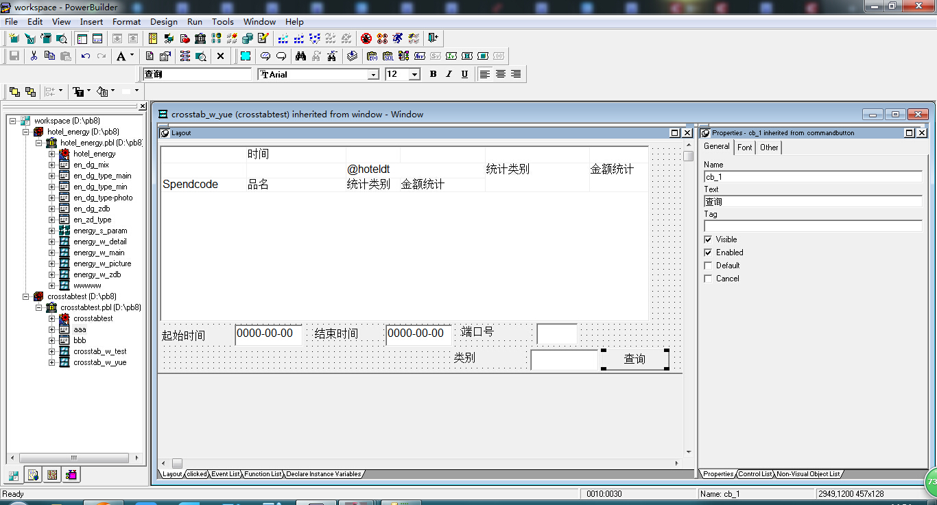
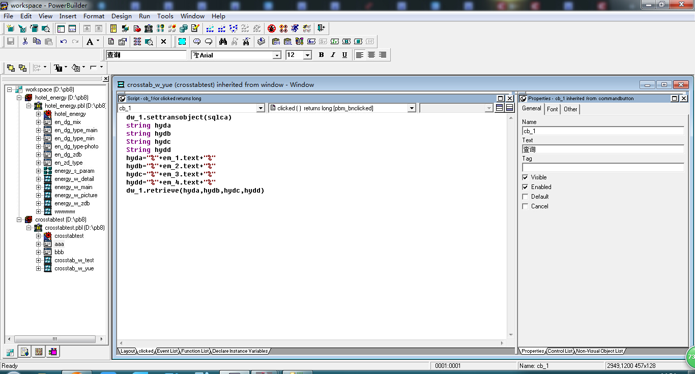
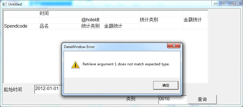
Retrieve argument 1 does not match expected type

bufenbaizhou 2015-04-01 02:57:33

在保存的click事件中 写入 最后提示
感谢解答 万谢万谢
...全文
641 1 打赏 收藏 转发到动态 举报
写回复
用AI写文章
1 条回复
切换为时间正序
请发表友善的回复…
发表回复
fengxiaohan211 2015-04-02
  • 打赏
  • 举报
回复
是模糊查询?应该是你的参数的检索类型不一致
sdk LCS/Telegraphics Wintab* Interface Specification 1.1: 16- and 32-bit API Reference By Rick Poyner Revised February 11, 2012 This specification was developed in response to a perceived need for a standardized programming inter-face to digitizing tablets, three dimensional position sensors, and other pointing devices by a group of lead-ing digitizer manufacturers and applications developers. The availability of drivers that support the features of the specification will simplify the process of developing Windows appli¬cation programs that in-corporate absolute coordinate input, and enhance the acceptance of ad¬vanced pointing de¬vices among users. This specification is intended to be an open standard, and as such the text and information contained herein may be freely used, copied, or distributed without compensation or licensing restrictions. This document is copyright 1991-2012 by LCS/Telegraphics.* Address questions and comments to: LCS/Telegraphics 150 Rogers St. Cambridge, MA 02142 (617)225-7970 (617)225-7969 FAX Compuserve: 76506,1676 Internet: wintab@pointing.com Note: sections marked with the “(1.1)” are new sections added for specification version 1.1. Sec-tions bearing the “(1.1 modified)” notation contain updated information for specification version 1.1. Version 1.1 Update Notation Conventions 1 1. Background Information 1 1.1. Features of Digitizers 1 1.2. The Windows Environment 1 2. Design Goals 2 2.1. User Control 2 2.2. Ease of Programming 2 2.3. Tablet Sharing 3 2.4. Tablet Feature Support 3 3. Design Concepts 3 3.1. Device Conventions 3 3.2. Device Information 4 3.3. Tablet Contexts 4 3.4. Event Packets 4 3.5. Tablet Managers 5 3.6. Extensions 5 3.7. Persistent Binding of Interface Features (1.1) 6 4. Interface Implementations 6 4.1. File and Module Conventions 6 4.2. Feature Support Options 6 5. Function Reference 7 5.1. Basic Functions 7 5.1.1. WTInfo 8 5.1.2. WTOpen 9 5.1.3. WTClose 10 5.1.4. WTPacketsGet 10 5.1.5. WTPacket 11 5.2. Visibility Functions 11 5.2.1. WTEnable 11 5.2.2. WTOverlap 12 5.3. Context Editing Functions 12 5.3.1. WTConfig 12 5.3.2. WTGet 13 5.3.3. WTSet (1.1 modified) 13 5.3.4. WTExtGet 14 5.3.5. WTExtSet 14 5.3.6. WTSave 15 5.3.7. WTRestore 15 5.4. Advanced Packet and Queue Functions 16 5.4.1. WTPacketsPeek 16 5.4.2. WTDataGet 17 5.4.3. WTDataPeek 17 5.4.4. WTQueuePackets (16-bit only) 18 5.4.5. WTQueuePacketsEx 18 5.4.6. WTQueueSizeGet 19 5.4.7. WTQueueSizeSet 19 5.5. Manager Handle Functions 19 5.5.1. WTMgrOpen 19 5.5.2. WTMgrClose 20 5.6. Manager Context Functions 20 5.6.1. WTMgrContextEnum 20 5.6.2. WTMgrContextOwner 21 5.6.3. WTMgrDefContext 22 5.6.4. WTMgrDefContextEx (1.1) 22 5.7. Manager Configuration Functions 23 5.7.1. WTMgrDeviceConfig 23 5.7.2. WTMgrConfigReplace (16-bit only) 24 5.7.3. WTMgrConfigReplaceEx 24 5.8. Manager Packet Hook Functions 25 5.8.1. WTMgrPacketHook (16-bit only) 26 5.8.2. WTMgrPacketHookEx 26 5.8.3. WTMgrPacketUnhook 29 5.8.4. WTMgrPacketHookDefProc (16-bit only) 30 5.8.5. WTMgrPacketHookNext 30 5.9. Manager Preference Data Functions 31 5.9.1. WTMgrExt 31 5.9.2. WTMgrCsrEnable 32 5.9.3. WTMgrCsrButtonMap 32 5.9.4. WTMgrCsrPressureBtnMarks (16-bit only) 33 5.9.5. WTMgrCsrPressureBtnMarksEx 33 5.9.6. WTMgrCsrPressureResponse 34 5.9.7. WTMgrCsrExt 35 6. Message Reference 36 6.1. Event Messages 36 6.1.1. WT_PACKET 36 6.1.2. WT_CSRCHANGE (1.1) 37 6.2. Context Messages 37 6.2.1. WT_CTXOPEN 37 6.2.2. WT_CTXCLOSE 37 6.2.3. WT_CTXUPDATE 38 6.2.4. WT_CTXOVERLAP 38 6.2.5. WT_PROXIMITY 38 6.3. Information Change Messages 39 6.3.1. WT_INFOCHANGE 39 7. Data Reference 39 7.1. Common Data Types (1.1 modified) 39 7.2. Information Data Structures 41 7.2.1. AXIS 41 7.2.2. Information Categories and Indices (1.1 modified) 42 7.3. Context Data Structures 50 7.3.1. LOGCONTEXT (1.1 modified) 50 7.4. Event Data Structures 55 7.4.1. PACKET (1.1 modified) 55 7.4.2. ORIENTATION 57 7.4.3. ROTATION (1.1) 58 Appendix A. Using PKTDEF.H 59 Appendix B. Extension Definitions 60 B.1. Extensions Programming 60 B.2. Out of Bounds Tracking 61 OBT Programming 61 Information Category 61 Turning OBT On and Off 61 B.3. Function Keys 62 FKEYS Programming 62 Information Category 62 B.4. Tilt 62 TILT Programming 63 Information Category 63 B.5. Cursor Mask 63 CSRMASK Programming 64 Information Category 64 B.6. Extended Button Masks 64 XBTNMASK Programming 64 Information Category 65 VERSION 1.1 UPDATE NOTATION CONVENTIONS Sections marked with the “(1.1)” are new sections added for specification version 1.1. Sections bearing the “(1.1 modified)” notation contain updated information for specification version 1.1. The “(1.1)” notation also marks the definitions of new functions, messages, and data structures. The nota-tion “1.1:” marks new text or commentaries explaining new functionality added to existing features. 1 BACKGROUND INFORMATION This document describes a programming interface for using digitizing tablets and other advanced pointing de¬vices with Microsoft Windows Version 3.0 and above. The design presented here is based on the input of numerous professionals from the pointing device manufacturing and Windows soft¬ware development industries. In this document, the words "tablet" and "digitizer" are used interchange¬ably to mean all absolute point¬ing or digitizing devices that can be made to work with this interface. The definition is not lim¬ited to de¬vices that use a physical tablet. In fact, this specification can support de¬vices that combine rela¬tive and absolute pointing as well as purely relative devices. The following sections describe features of tablets and of the Windows environment that helped mo¬tivate the design. 1.1 Features of Digitizers Digitizing tablets present several problems to device interface authors. • Many tablets have a very high report rate. • Many tablets have many configurable features and types of input information. • Tablets often control the system cursor, provide additional digitizing input, and provide template or macro functions. 1.2 The Windows Environment Programming for tablets in the Windows environment presents additional problems. • Multitasking means multiple applications may have to share the tablet. • The tablet must also be able to control the system cursor and/or the pen (in Pen Windows). • The tablet must work with legacy applications, and with applications written to take advan¬tage of tablet services. • The tablet driver must add minimal speed and memory overhead, so as many applications as possible can run as efficiently as possible. • The user should be able to control how applications use the tablet. The user interface must be ef-ficient, consistent, and customizable. 2 DESIGN GOALS While the tablet interface design must address the technical problems stated above, it must also be useful to the programmers who will write tablet programs, and ultimately, to the tablet users. Four design goals will help clarify these needs, and provide some criteria for evaluating the interface speci¬fication. The goals are user control, ease of programming, tablet sharing, and tablet feature support. 2.1 User Control The user should be able to use and control the tablet in as natural and easy a manner as possible. The user's preferences should take precedence over application requests, where possible. Here are questions to ask when thinking about user control as a design goal: • Can the user understand how applications use the tablet? • Is the interface for controlling tablet functions natural and unobtrusive? • Is the user allowed to change things that help to customize the work environment, but pre¬vented from changing things over which applications must have control? 2.2 Ease of Programming Programming is easiest when the amount of knowledge and effort required matches the task at hand. Writing simple programs should require only a few lines of code and a minimal understanding of the en-vironment. On the other hand, more advanced features and functions should be available to those who need them. The interface should accommodate three kinds of programmers: those who wish to write sim-ple tablet programs, programmers who wish to write complex applications that take full ad¬vantage of tab-let capabilities, and programmers who wish to provide tablet device control features. In addition, the inter-face should accommodate programmers in as many different programming lan¬guages, situations, and en-vironments as possible. Questions to ask when thinking about ease of programming include: • How hard is it to learn the interface and write a simple program that uses tablet input? • Can programmers of complex applications control the features they need? • Are more powerful tablet device control features available? • Can the interface be used in different programming environments? • Is the interface logical, consistent, and robust? 2.3 Tablet Sharing In the Windows environment, multiple applications that use the tablet may be running at once. Each ap-plication will require different services. Applications must be able to get the services they need without getting in each others' way. Questions to ask when thinking about tablet sharing include: • Can tablet applications use the tablet features they need, independent of other applications? • Does the interface prevent a rogue application from "hijacking" the tablet, or causing dead¬locks? • Does the sharing architecture promote efficiency? 2.4 Tablet Feature Support The interface gives standard access to as many features as possible, while leaving room for future ex¬ten-sions and vendor-specific customizations. Applications should be able to get the tablet informa¬tion and services they want, just the way they want them. Users should be able to use the tablet to set up an effi-cient, comfortable work environment. Questions to ask when thinking about tablet feature support include: • Does the interface provide the features applications need? Are any commonly available fea¬tures not supported? • Does the interface provide what users need? Is anything missing? • Are future extensions possible and fairly easy? • Are vendor-specific extensions possible? 3 DESIGN CONCEPTS The proposed interface design depends on several fundamental concepts. Devices and cursor types de-scribe physical hardware configurations. The interface publishes read-only information through a single information interface. Applications interact with the interface by setting up tablet contexts and consuming event packets. Applications may assume interface and hardware control functions by be¬coming tablet managers. The interface provides explicit support for future extensions. 3.1 Device Conventions The interface provides access to one or more devices that produce pointing input. Devices sup¬ported by this interface have some common characteristics. The device must define an absolute or relative coordi-nate space in at least two dimensions for which it can return position data. The device must have a point-ing ap¬para¬tus or method (such as a stylus, or a finger touching a touch pad), called the cursor, that de¬fines the current position. The cursor must be able to return at least one bit of additional state (via a but¬ton, touching a digitizing surface, etc.). Devices may have multiple cursor types that have different physical configurations, or that have differ¬ent numbers of buttons, or return auxiliary information, such as pressure information. Cursor types may also describe different optional hardware configurations. The interface defines a standard orientation for reporting device native coordinates. When the user is viewing the device in its normal position, the coordinate origin will be at the lower left of the device. The coordinate system will be right-handed, that is, the positive x axis points from left to right, and the posi¬tive y axis points either upward or away from the user. The z axis, if supported, points either to¬ward the user or upward. For devices that lay flat on a table top, the x-y plane will be horizontal and the z axis will point upward. For devices that are oriented vertically (for example, a touch screen on a conventional dis¬play), the x-y plane will be vertical, and the z axis will point toward the user. 3.2 Device Information Any program can get descriptive information about the tablet via the WTInfo function. The interface specifies certain information that must be available, but allows new implementations to add new types of information. The basic information includes device identifiers, version numbers, and overall ca¬pabilities. The information items are organized by category and index numbers. The combination of a category and index specifies a single information data item, which may be a scalar value, string, structure, or array. Applica¬tions may retrieve single items or whole categories at once. Some categories are multiplexed. A single category code represents the first of a group of identically in-dexed categories, one for each of a set of similar objects. Multiplexed categories in¬clude those for devices and cur¬sor types. One constructs the category number by adding the defined cate¬gory code to a zero-based device or cursor identification number. The information is read-only for normal tablet applications. Some information items may change during the course of a Windows session; tablet applications receive messages notifying them of changes in tablet information. 3.3 Tablet Contexts Tablet contexts play a central role in the interface; they are the objects that applications use to specify their use of the tablet. Con¬texts include not only the physical area of the tablet that the application will use, but also information about the type, con¬tents, and delivery method for tablet events, as well as other information. Tablet contexts are somewhat analo¬gous to display contexts in the GDI interface model; they contain context information about a spe¬cific application's use of the tablet. An application can open more than one context, but most only need one. Applications can customize their contexts, or they can open a context using a default context specification that is always available. The WTInfo function provides access to the default context specification. Opening a context requires a window handle. The window handle becomes the context's owner and will receive any window messages associated with the context. Contexts are remotely similar to screen windows in that they can physically overlap. The tablet inter¬face uses a combination of context overlap order and context attributes to decide which context will process a given event. The topmost context in the overlap order whose input context encompasses the event, and whose event masks select the event, will process the event. (Note that the notion of overlap order is sepa-rate from the notion of the physical z dimension.) Tablet managers (described below) provide a way to modify and overlap contexts. 3.4 Event Packets Tablet contexts generate and report tablet activity via event packets. Applications can control how they receive events, which events they receive, and what information they contain. Applications may receive events either by polling, or via Windows messages. • Polling: Any application that has opened a context can call the WTPacketsGet function to get the next state of the tablet for that context. • Window Messages: Applications that request messages will receive the WT_PACKET mes¬sage (described below), which indicates that something happened in the context and provides a refer-ence to more information. Applications can control which events they receive by using event masks. For example, some appli¬ca¬tions may only need to know when a button is pressed, while others may need to receive an event every time the cursor moves. Tablet context event masks implement this type of control. Applications can control the contents of the event packets they receive. Some tablets can return data that many applications will not need, like button pressure and three dimensional position and orien¬tation in-formation. The context object provides a way of specifying which data items the appli¬cation needs. This allows the driver to improve the efficiency of packet delivery to applications that only need a few items per packet. Packets are stored in context-specific packet queues and retrieved by explicit function calls. The interface provides ways to peek at and get packets, to query the size and contents of the queue, and to re-size the queue. 3.5 Tablet Managers The interface provides functions for tablet management. An application can become a tablet manager by opening a tablet manager handle. This handle allows the manager access to spe¬cial functions. These man-agement functions allow the application to arrange, overlap, and modify tablet contexts. Man¬agers may also perform other functions, such as changing default values used by applica¬tions, chang¬ing ergo¬nomic, preference, and configuration settings, controlling tablet behavior with non-tablet aware applica¬tions, modi¬fy¬ing user dialogs, and recording and playing back tablet packets. Opening a manager handle re¬quires a window handle. The window becomes a manager window and receives window messages about interface and con¬text activity. 3.6 Extensions The interface allows implementations to define additional features called extensions. Extensions can be made available to new applications without the need to modify ex¬isting applications. Extensions are sup-ported through the information categories, through the flexible definition of packets, and through special context and manager functions. Designing an extension involves defining the meaning and behavior of the extension packet and/or prefer-ence data, filling in the information category, defining the extension's interface with the special functions, and possibly defining additional functions to support the extension. Each extension will be assigned a unique tag for identification. Not all implementations will support all extensions. A multiplexed information category contains descriptive data about extensions. Note that applica¬tions must find their extensions by iterating through the categories and matching tags. While tags are fixed across all implementations, category numbers may vary among implementations. 3.7 Persistent Binding of Interface Features (1.1) The interface provides access to many of its features using consecutive numeric indices whose value is not guaranteed from session to session. However, sufficient information is provided to create unique identifi¬ers for devices, cursors, and interface extensions. Devices should be uniquely identified by the contents of their name strings. If multiple identical devices are present, implementation providers should provide unique, persistent id strings to the extent possible. Identical devices that return unique serial numbers are ideal. If supported by the hardware, cursors also may have a physical cursor id that uniquely identifies the cursor in a persistent and stable manner. Interface extensions are uniquely identified by their tag. 4 INTERFACE IMPLEMENTATIONS Implementations of this interface usually support one specific device, a class of similar devices, or a com-mon combination of devices. The following sections discuss guidelines for implementations. 4.1 File and Module Conventions For 16-bit implementations, the interface functions, and any additional vendor- or device-specific func-tions, reside in a dynamic link library with the file name "WINTAB.DLL" and module name "WINTAB"; 32-bit implementations use the file name "WINTAB32.DLL" and module name "WINTAB32." Any other file or module con¬ventions are implementation specific. Implementations may include other library mod-ules or data files as necessary. Installation processes are likewise implementa¬tion-specific. Wintab programs written in the C language require two header files. WINTAB.H contains definitions of all of the functions, constants, and fixed data types. PKTDEF.H contains a parameterized definition of the PACKET data structure, that can be tailored to fit the application. The Wintab Programmer's Kit con¬tains these and other files necessary for Wintab programming, plus several example programs with C-lan¬guage source files. The Wintab Programmer's Kit is available from the author. 4.2 Feature Support Options Some features of the interface are optional and may be left out by some implementations. Support of defined data items other than x, y, and buttons is optional. Many devices only report x, y, and button information. Support of system-cursor contexts is optional. This option relieves implementations of replacing the sys¬tem mouse driver in Windows versions before 3.1. Support of Pen Windows contexts is optional. Not all systems will have the Pen Windows hardware and software necessary. Support of external tablet manager applications is optional, and the number of manager handles is imple-mentation-dependent. However, the manager functions should be present in all implementa¬tions, return¬ing appropriate failure codes if not fully implemented. An implementation may provide context- and hardware-management support internally only, if desired. On the other hand, providing the external man-ager interface may relieve the implementation of a considerable amount of user in¬terface code, and make improvements to the manager interface easier to implement and distribute later. Support of extension data items is optional. Most extensions will be geared to unusual hardware features. 5 FUNCTION REFERENCE All tablet function names have the prefix "WT" and have attributes equivalent to WINAPI. Applica¬tions gain access to the tablet interface functions through a dynamic-link library with standard file and module names, as defined in the previous section. Applications may link to the functions by using the Windows functions LoadLibrary, FreeLibrary, and GetProcAddress, or use an import library. Specific to 32-bit Wintab: The functions WTInfo, WTOpen, WTGet, and WTSet have both ANSI and Unicode versions, using the same ANSI/Unicode porting conventions used in the Win32 API. Five non-portable functions, WTQueuePackets, WTMgrCsrPressureBtnMarks, WTMgrConfigReplace, WTMgrPacketHook, and WTMgrPacketHookDefProc are replaced by new portable functions WTQueuePacketsEx, WTMgrCsrPressureBtnMarksEx, WTMgrConfigReplaceEx, WTMgrPack-etHookEx, WTMgrPacketUnhook, and WTMgrPacketHookNext. WTMgrConfigReplaceEx and WTMgrPacketHookEx have both ANSI and Unicode versions. Table 5.1. Ordinal Function Numbers for Dynamic Linking Ordinal numbers for dynamic linking are defined in the table below. Where two ordinal entries appear, the first entry identifies the 16-bit and 32-bit ANSI versions of the function. The second entry identifies the 32-bit Unicode version. Function Name Ordinal Function Name Ordinal WTInfo 20, 1020 WTMgrOpen 100 WTOpen 21, 1021 WTMgrClose 101 WTClose 22 WTMgrContextEnum 120 WTPacketsGet 23 WTMgrContextOwner 121 WTPacket 24 WTMgrDefContext 122 WTEnable 40 WTMgrDefContextEx (1.1) 206 WTOverlap 41 WTMgrDeviceConfig 140 WTConfig 60 WTMgrConfigReplace 141 WTGet 61, 1061 WTMgrConfigReplaceEx 202, 1202 WTSet 62, 1062 WTMgrPacketHook 160 WTExtGet 63 WTMgrPacketHookEx 203, 1203 WTExtSet 64 WTMgrPacketUnhook 204 WTSave 65 WTMgrPacketHookDefProc 161 WTRestore 66 WTMgrPacketHookNext 205 WTPacketsPeek 80 WTMgrExt 180 WTDataGet 81 WTMgrCsrEnable 181 WTDataPeek 82 WTMgrCsrButtonMap 182 WTQueuePackets 83 WTMgrCsrPressureBtnMarks 183 WTQueuePacketsEx 200 WTMgrCsrPressureBtnMarksEx 201 WTQueueSizeGet 84 WTMgrCsrPressureResponse 184 WTQueueSizeSet 85 WTMgrCsrExt 185 5.1 Basic Functions The functions in the following section will be used by most tablet-aware applications. They include getting interface and device information, opening and closing contexts, and retrieving packets by polling or via Windows messages. 5.1.1 WTInfo Syntax UINT WTInfo(wCategory, nIndex, lpOutput) This function returns global information about the interface in an application-sup-plied buffer. Different types of information are specified by different index argu-ments. Applications use this function to receive information about tablet coordi-nates, physical dimensions, capabilities, and cursor types. Parameter Type/Description wCategory UINT Identifies the category from which information is being re-quested. nIndex UINT Identifies which information is being requested from within the category. lpOutput LPVOID Points to a buffer to hold the requested information. Return Value The return value specifies the size of the returned information in bytes. If the infor-mation is not supported, the function returns zero. If a tablet is not physi¬cally pres-ent, this function always returns zero. Comments Several important categories of information are available through this function. First, the function provides identification information, including specification and software version numbers, and tablet vendor and model information. Sec¬ond, the function provides general capability information, including dimensions, resolutions, optional features, and cursor types. Third, the function provides categories that give defaults for all tablet context attributes. Finally, the func¬tion may provide any other implementation- or vendor-specific information cat¬egories necessary. The information returned by this function is subject to change during a Win¬dows session. Applications cannot change the information returned here, but tablet man-ager applications or hardware changes or errors can. Applications can respond to information changes by fielding the WT_INFOCHANGE message. The parameters of the message indicate which information has changed. If the wCategory argument is zero, the function copies no data to the output buffer, but returns the size in bytes of the buffer necessary to hold the largest complete category. If the nIndex argument is zero, the function returns all of the information entries in the category in a single data structure. If the lpOutput argument is NULL, the function just returns the required buffer size. See Also Category and index definitions in tables 7.3 through 7.9, and the WT_INFOCHANGE message in section 6.3.1. 5.1.2 WTOpen Syntax HCTX WTOpen(hWnd, lpLogCtx, fEnable) This function establishes an active context on the tablet. On successful comple¬tion of this function, the application may begin receiving tablet events via mes¬sages (if they were requested), and may use the handle returned to poll the con¬text, or to per-form other context-related functions. Parameter Type/Description hWnd HWND Identifies the window that owns the tablet context, and receives messages from the context. lpLogCtx LPLOGCONTEXT Points to an application-provided LOGCONTEXT data structure describing the context to be opened. fEnable BOOL Specifies whether the new context will immediately begin processing input data. Return Value The return value identifies the new context. It is NULL if the context is not opened. Comments Opening a new context allows the application to receive tablet input or creates a context that controls the system cursor or Pen Windows pen. The owning window (and all manager windows) will immediately receive a WT_CTXOPEN message when the context has been opened. If the fEnable argument is zero, the context will be created, but will not process input. The context can be enabled using the WTEnable function. If tablet event messages were requested in the context specification, the owning window will receive them. The application can control the message numbers used the lcMsgBase field of the LOGCONTEXT structure. The window that owns the new context will receive context and information change messages even if event messages were not requested. It is not necessary to handle these in many cases, but some applications may wish to do so. The newly opened tablet context will be placed on the top of the context overlap or-der. Invalid or out-of-range attribute values in the logical context structure will ei¬ther be validated, or cause the open to fail, depending on the attributes involved. Upon a successful return from the function, the context specification pointed to by lpLogCtx will contain the validated values. See Also The WTEnable function in section 5.2.1, the LOGCONTEXT data structure in section 7.3.1, and the context and infor¬mation change messages in sections 6.2 and 6.3. 5.1.3 WTClose Syntax BOOL WTClose(hCtx) This function closes and destroys the tablet context object. Parameter Type/Description hCtx HCTX Identifies the context to be closed. Return Value The function returns a non-zero value if the context was valid and was destroyed. Otherwise, it returns zero. Comments After a call to this function, the passed handle is no longer valid. The owning win¬dow (and all manager windows) will receive a WT_CTXCLOSE message when the context has been closed. See Also The WTOpen function in section 5.1.2. 5.1.4 WTPacketsGet Syntax int WTPacketsGet(hCtx, cMaxPkts, lpPkts) This function copies the next cMaxPkts events from the packet queue of context hCtx to the passed lpPkts buffer and removes them from the queue. Parameter Type/Description hCtx HCTX Identifies the context whose packets are being returned. cMaxPkts int Specifies the maximum number of packets to return. lpPkts LPVOID Points to a buffer to receive the event packets. Return Value The return value is the number of packets copied in the buffer. Comments The exact structure of the returned packet is determined by the packet infor¬mation that was requested when the context was opened. The buffer pointed to by lpPkts must be at least cMaxPkts * sizeof(PACKET) bytes long to prevent overflow. Applications may flush packets from the queue by calling this function with a NULL lpPkt argument. See Also The WTPacketsPeek function in section 5.4.1, and the descriptions of the LOGCONTEXT (section 7.3.1) and PACKET (section 7.4.1) data structures. 5.1.5 WTPacket Syntax BOOL WTPacket(hCtx, wSerial, lpPkt) This function fills in the passed lpPkt buffer with the context event packet having the specified serial number. The returned packet and any older packets are removed from the context's internal queue. Parameter Type/Description hCtx HCTX Identifies the context whose packets are being returned. wSerial UINT Serial number of the tablet event to return. lpPkt LPVOID Points to a buffer to receive the event packet. Return Value The return value is non-zero if the specified packet was found and returned. It is zero if the specified packet was not found in the queue. Comments The exact structure of the returned packet is determined by the packet infor¬mation that was requested when the context was opened. The buffer pointed to by lpPkts must be at least sizeof(PACKET) bytes long to pre-vent overflow. Applications may flush packets from the queue by calling this function with a NULL lpPkts argument. See Also The descriptions of the LOGCONTEXT (section 7.3.1) and PACKET (section 7.4.1) data structures. 5.2 Visibility Functions The functions in this section allow applications to control contexts' visibility, whether or not they are pro-cessing input, and their overlap order. 5.2.1 WTEnable Syntax BOOL WTEnable(hCtx, fEnable) This function enables or disables a tablet context, temporarily turning on or off the processing of packets. Parameter Type/Description hCtx HCTX Identifies the context to be enabled or disabled. fEnable BOOL Specifies enabling if non-zero, disabling if zero. Return Value The function returns a non-zero value if the enable or disable request was satis¬fied, zero otherwise. Comments Calls to this function to enable an already enabled context, or to disable an al¬ready disabled context will return a non-zero value, but otherwise do nothing. The context’s packet queue is flushed on disable. Applications can determine whether a context is currently enabled by using the WTGet function and examining the lcStatus field of the LOGCONTEXT struc¬ture. See Also The WTGet function in section 5.3.2, and the LOGCONTEXT structure in sec¬tion 7.3.1. 5.2.2 WTOverlap Syntax BOOL WTOverlap(hCtx, fToTop) This function sends a tablet context to the top or bottom of the order of over¬lapping tablet contexts. Parameter Type/Description hCtx HCTX Identifies the context to move within the overlap order. fToTop BOOL Specifies sending the context to the top of the overlap or-der if non-zero, or to the bottom if zero. Return Value The function returns non-zero if successful, zero otherwise. Comments Tablet contexts' input areas are allowed to overlap. The tablet interface main¬tains an overlap order that helps determine which context will process a given event. The topmost context in the overlap order whose input context encom¬passes the event, and whose event masks select the event will process the event. This function is useful for getting access to input events when the application's con-text is overlapped by other contexts. The function will fail only if the context argument is invalid. 5.3 Context Editing Functions This group of functions allows applications to edit, save, and restore contexts. 5.3.1 WTConfig Syntax BOOL WTConfig(hCtx, hWnd) This function prompts the user for changes to the passed context via a dialog box. Parameter Type/Description hCtx HCTX Identifies the context that the user will modify via the dialog box. hWnd HWND Identifies the window that will be the parent window of the dialog box. Return Value The function returns a non-zero value if the tablet context was changed, zero oth-erwise. Comments Tablet applications can use this function to let the user choose context attributes that the application doesn't need to control. Applications can control the editing of con¬text attributes via the lcLocks logical context structure member. Applications should consider providing access to this function through a menu item or command. See Also The LOGCONTEXT structure in section 7.3.1 and the context lock values in table 7.13. 5.3.2 WTGet Syntax BOOL WTGet(hCtx, lpLogCtx) This function fills the passed structure with the current context attributes for the passed handle. Parameter Type/Description hCtx HCTX Identifies the context whose attributes are to be copied. lpLogCtx LPLOGCONTEXT Points to a LOGCONTEXT data structure to which the context attributes are to be copied. Return Value The function returns a non-zero value if the data is retrieved successfully. Oth¬er¬wise, it returns zero. See Also The LOGCONTEXT structure in section 7.3.1. 5.3.3 WTSet (1.1 modified) Syntax BOOL WTSet(hCtx, lpLogCtx) This function allows some of the context's attributes to be changed on the fly. Parameter Type/Description hCtx HCTX Identifies the context whose attributes are being changed. lpLogCtx LPLOGCONTEXT Points to a LOGCONTEXT data structure containing the new context attributes. Return Value The function returns a non-zero value if the context was changed to match the passed context specification; it returns zero if any of the requested changes could not be made. Comments If this function is called by the task or process that owns the context, any context attribute may be changed. Otherwise, the function can change attributes that do not affect the format or meaning of the context's event packets and that were not speci-fied as locked when the context was opened. Context lock values can only be changed by the context’s owner. 1.1: If the hCtx argument is a default context handle returned from WTMgrDef-Context or WTMgrDefContextEx, and the lpLogCtx argument is WTP_LPDEFAULT, the default context will be reset to its initial factory default values. See Also The LOGCONTEXT structure in section 7.3.1 and the context lock values in table 7.13. 5.3.4 WTExtGet Syntax BOOL WTExtGet(hCtx, wExt, lpData) This function retrieves any context-specific data for an extension. Parameter Type/Description hCtx HCTX Identifies the context whose extension attributes are being retrieved. wExt UINT Identifies the extension tag for which context-specific data is being retrieved. lpData LPVOID Points to a buffer to hold the retrieved data. Return Value The function returns a non-zero value if the data is retrieved successfully. Oth¬er¬wise, it returns zero. See Also The extension definitions in Appendix B. 5.3.5 WTExtSet Syntax BOOL WTExtSet(hCtx, wExt, lpData) This function sets any context-specific data for an extension. Parameter Type/Description hCtx HCTX Identifies the context whose extension attributes are being modified. wExt UINT Identifies the extension tag for which context-specific data is being modified. lpData LPVOID Points to the new data. Return Value The function returns a non-zero value if the data is modified successfully. Oth¬er¬wise, it returns zero. Comments Extensions may forbid their context-specific data to be changed during the life¬time of a context. For such extensions, calls to this function would always fail. Extensions may also limit context data editing to the task of the owning window, as with the context locks. See Also The extension definitions in Appendix B, the LOGCONTEXT data structure in section 7.3.1 and the context locking values in table 7.13. 5.3.6 WTSave Syntax BOOL WTSave(hCtx, lpSaveInfo) This function fills the passed buffer with binary save information that can be used to restore the equivalent context in a subsequent Windows session. Parameter Type/Description hCtx HCTX Identifies the context that is being saved. lpSaveInfo LPVOID Points to a buffer to contain the save information. Return Value The function returns non-zero if the save information is successfully retrieved. Oth-erwise, it returns zero. Comments The size of the save information buffer can be determined by calling the WTInfo function with category WTI_INTERFACE, index IFC_CTXSAVESIZE. The save information is returned in a private binary data format. Applications should store the information unmodified and recreate the context by passing the save information to the WTRestore function. Using WTSave and WTRestore allows applications to easily save and restore ex-tension data bound to contexts. See Also The WTRestore function in section 5.3.7. 5.3.7 WTRestore Syntax HCTX WTRestore(hWnd, lpSaveInfo, fEnable) This function creates a tablet context from save information returned from the WTSave function. Parameter Type/Description hWnd HWND Identifies the window that owns the tablet context, and receives messages from the context. lpSaveInfo LPVOID Points to a buffer containing save information. fEnable BOOL Specifies whether the new context will immediately begin processing input data. Return Value The function returns a valid context handle if successful. If a context equivalent to the save information could not be created, the function returns NULL. Comments The save information is in a private binary data format. Applications should only pass save information retrieved by the WTSave function. This function is much like WTOpen, except that it uses save in¬formation for input instead of a logical context. In particular, it will generate a WT_CTXOPEN mes¬sage for the new context. See Also The WTOpen function in section 5.1.2, the WTSave function in section 5.3.6, and the WT_CTXOPEN message in section 6.2.1. 5.4 Advanced Packet and Queue Functions These functions provide advanced packet retrieval and queue manipulation. The packet retrieval functions require the application to provide a packet output buffer. To prevent overflow, the buffer must be large enough to hold the requested number of packets from the specified context. It is up to the caller to deter¬mine the packet size (by interrogating the context, if necessary), and to allocate a large enough buffer. Ap¬plications may flush packets from the queue by passing a NULL buffer pointer. 5.4.1 WTPacketsPeek Syntax int WTPacketsPeek(hCtx, cMaxPkts, lpPkts) This function copies the next cMaxPkts events from the packet queue of context hCtx to the passed lpPkts buffer without removing them from the queue. Parameter Type/Description hCtx HCTX Identifies the context whose packets are being read. cMaxPkts int Specifies the maximum number of packets to return. lpPkts LPVOID Points to a buffer to receive the event packets. Return Value The return value is the number of packets copied in the buffer. Comments The buffer pointed to by lpPkts must be at least cMaxPkts * sizeof(PACKET) bytes long to prevent overflow. See Also the WTPacketsGet function in section 5.1.4. 5.4.2 WTDataGet Syntax int WTDataGet(hCtx, wBegin, wEnd, cMaxPkts, lpPkts, lpNPkts) This function copies all packets with serial numbers between wBegin and wEnd in-clusive from the context's queue to the passed buffer and removes them from the queue. Parameter Type/Description hCtx HCTX Identifies the context whose packets are being returned. wBegin UINT Serial number of the oldest tablet event to return. wEnd UINT Serial number of the newest tablet event to return. cMaxPkts int Specifies the maximum number of packets to return. lpPkts LPVOID Points to a buffer to receive the event packets. lpNPkts LPINT Points to an integer to receive the number of packets ac-tually copied. Return Value The return value is the total number of packets found in the queue between wBegin and wEnd. Comments The buffer pointed to by lpPkts must be at least cMaxPkts * sizeof(PACKET) bytes long to prevent overflow. See Also The WTDataPeek function in section 5.4.3, and the WTQueuePacketsEx function in section 5.4.5. 5.4.3 WTDataPeek Syntax int WTDataPeek(hCtx, wBegin, wEnd, cMaxPkts, lpPkts, lpNPkts) This function copies all packets with serial numbers between wBegin and wEnd in-clusive, from the context's queue to the passed buffer without removing them from the queue. Parameter Type/Description hCtx HCTX Identifies the context whose packets are being read. wBegin UINT Serial number of the oldest tablet event to return. wEnd UINT Serial number of the newest tablet event to return. cMaxPkts int Specifies the maximum number of packets to return. lpPkts LPVOID Points to a buffer to receive the event packets. lpNPkts LPINT Points to an integer to receive the number of packets ac-tually copied. Return Value The return value is the total number of packets found in the queue between wBegin and wEnd. Comments The buffer pointed to by lpPkts must be at least cMaxPkts * sizeof(PACKET) bytes long to prevent overflow. See Also The WTDataGet function in section 5.4.2, and the WTQueuePacketsEx function in section 5.4.5. 5.4.4 WTQueuePackets (16-bit only) Syntax DWORD WTQueuePackets(hCtx) This function returns the serial numbers of the oldest and newest packets cur¬rently in the queue. Parameter Type/Description hCtx HCTX Identifies the context whose queue is being queried. Return Value The high word of the return value contains the newest packet's serial number; the low word contains the oldest. Comments This function is non-portable and is superseded by WTQueuePacketsEx. See Also The WTQueuePacketsEx function in section 5.4.5. 5.4.5 WTQueuePacketsEx Syntax BOOL WTQueuePacketsEx(hCtx, lpOld, lpNew) This function returns the serial numbers of the oldest and newest packets cur¬rently in the queue. Parameter Type/Description hCtx HCTX Identifies the context whose queue is being queried. lpOld UINT FAR * Points to an unsigned integer to receive the oldest packet's serial number. lpNew UINT FAR * Points to an unsigned integer to receive the newest packet's serial number. Return Value The function returns non-zero if successful, zero otherwise. 5.4.6 WTQueueSizeGet Syntax int WTQueueSizeGet(hCtx) This function returns the number of packets the context's queue can hold. Parameter Type/Description hCtx HCTX Identifies the context whose queue size is being re¬turned. Return Value The return value is the number of packet the queue can hold. See Also The WTQueueSizeSet function in section 5.4.7. 5.4.7 WTQueueSizeSet Syntax BOOL WTQueueSizeSet(hCtx, nPkts) This function attempts to change the context's queue size to the value specified in nPkts. Parameter Type/Description hCtx HCTX Identifies the context whose queue size is being set. nPkts int Specifies the requested queue size. Return Value The return value is non-zero if the queue size was successfully changed. Other¬wise, it is zero. Comments If the return value is zero, the context has no queue because the function deletes the original queue before attempting to create a new one. The application must continue calling the function with a smaller queue size until the function returns a non-zero value. See Also The WTQueueSizeGet function in section 5.4.6. 5.5 Manager Handle Functions The functions described in this and subsequent sections are for use by tablet manager applications. The functions of this section create and destroy manager handles. These handles allow the interface code to limit the degree of simultaneous access to the powerful manager functions. Also, opening a manager handle lets the application receive messages about tablet interface activity. 5.5.1 WTMgrOpen Syntax HMGR WTMgrOpen(hWnd, wMsgBase) This function opens a tablet manager handle for use by tablet manager and con¬figu-ration applications. This handle is required to call the tablet management func¬tions. Parameter Type/Description hWnd HWND Identifies the window which owns the manager handle. wMsgBase UINT Specifies the message base number to use when notifying the manager window. Return Value The function returns a manager handle if successful, otherwise it returns NULL. Comments While the manager handle is open, the manager window will receive context mes-sages from all tablet contexts. Manager windows also receive information change messages. The number of manager handles available is interface implementation-dependent, and can be determined by calling the WTInfo function with category WTI_INTERFACE and index IFC_NMANAGERS. See Also The WTInfo function in section 5.1.1, the WTMgrClose function in section 5.5.2, the description of message base numbers in section 6 and the context and in¬for¬ma-tion change messages in sections 6.2 and 6.3. 5.5.2 WTMgrClose Syntax BOOL WTMgrClose(hMgr) This function closes a tablet manager handle. After this function returns, the passed manager handle is no longer valid. Parameter Type/Description hMgr HMGR Identifies the manager handle to close. Return Value The function returns non-zero if the handle was valid; otherwise, it returns zero. 5.6 Manager Context Functions These functions provide access to all open contexts and their owners, and allow changing context de¬faults. Only tablet managers are allowed to manipulate tablet contexts belonging to other applica¬tions. 5.6.1 WTMgrContextEnum Syntax BOOL WTMgrContextEnum(hMgr, lpEnumFunc, lParam) This function enumerates all tablet context handles by passing the handle of each context, in turn, to the callback function pointed to by the lpEnumFunc pa¬rameter. The enumeration terminates when the callback function returns zero. Parameter Type/Description hMgr HMGR Is the valid manager handle that identifies the caller as a manager application. lpEnumFunc WTENUMPROC Is the procedure-instance address of the call-back function. See the following "Comments" section for details. lParam LPARAM Specifies the value to be passed to the callback func-tion for the application's use. Return Value The return value specifies the outcome of the function. It is non-zero if all con¬texts have been enumerated. Otherwise, it is zero. Comments The address passed as the lpEnumFunc parameter must be created by using the MakeProcInstance function. The callback function must have attributes equivalent to WINAPI. The callback function must have the following form: Callback BOOL WINAPI EnumFunc(hCtx, lParam) HCTX hCtx; LPARAM lParam; EnumFunc is a place holder for the application-supplied function name. The actual name must be exported by including it in an EXPORTS statement in the applica-tion's module-definition file. Parameter Description hCtx Identifies the context. lParam Specifies the 32-bit argument of the WTMgrContextEnum func-tion. Return Value The function must return a non-zero value to continue enumeration, or zero to stop it. 5.6.2 WTMgrContextOwner Syntax HWND WTMgrContextOwner(hMgr, hCtx) This function returns the handle of the window that owns a tablet context. Parameter Type/Description hMgr HMGR Is the valid manager handle that identifies the caller as a manager application. hCtx HCTX Identifies the context whose owner is to be returned. Return Value The function returns the context owner's window handle if the passed arguments are valid. Otherwise, it returns NULL. Comments This function allows the tablet manager to coordinate tablet context manage¬ment with the states of the context-owning windows. 5.6.3 WTMgrDefContext Syntax HCTX WTMgrDefContext(hMgr, fSystem) This function retrieves a context handle that allows setting values for the current default digit¬izing or system context. Parameter Type/Description hMgr HMGR Is the valid manager handle that identifies the caller as a manager application. fSystem BOOL Specifies retrieval of the default system context if non-zero, or the default digitizing context if zero. Return Value The return value is the context handle for the specified default context, or NULL if the arguments were invalid. Comments The default digitizing context is the context whose attributes are returned by the WTInfo function WTI_DEFCONTEXT category. The default system context is the context whose attributes are returned by the WTInfo function WTI_DEFSYSCTX category. Editing operations on the retrieved handles will fail if the new default contexts do not meet certain requirements. The digitizing context must include at least buttons, x, and y in its packet data, and must return absolute coordinates. 1.1: Editing the current default digitizing context will also update the device-spe¬cific default context for the device listed in the lcDevice field of the default con¬text’s LOGCONTEXT structure. See Also The WTInfo function in section 5.1.1 the WTMgrDefContextEx function in section 5.6.4, and the category and index definitions in tables 7.3 through 7.9. 5.6.4 WTMgrDefContextEx (1.1) Syntax HCTX WTMgrDefContextEx(hMgr, wDevice, fSystem) This function retrieves a context handle that allows setting values for the default digit¬izing or system context for a specified device. Parameter Type/Description hMgr HMGR Is the valid manager handle that identifies the caller as a manager application. wDevice UINT Specifies the device for which a default context handle will be returned. fSystem BOOL Specifies retrieval of the default system context if non-zero, or the default digitizing context if zero. Return Value The return value is the context handle for the specified default context, or NULL if the arguments were invalid. Comments The default digitizing contexts are contexts whose attributes are returned by the WTInfo function WTI_DDCTXS multiplexed category. The default system con-texts are contexts whose attributes are returned by the WTInfo function WTI_DSCTXS multiplexed category. Editing operations on the retrieved handles will fail if the new default contexts do not meet certain requirements. The digitizing context must include at least buttons, x, and y in its packet data, and must return absolute coordinates. See Also The WTInfo function in section 5.1.1, and the category and index definitions in tables 7.3 through 7.9. 5.7 Manager Configuration Functions These functions allow manager applications to replace the default context configuration dialog and to display a configuration dialog for each hardware device. 5.7.1 WTMgrDeviceConfig Syntax UINT WTMgrDeviceConfig(hMgr, wDevice, hWnd) This function displays a custom modal tablet-hardware configuration dialog box, if one is supported. Parameter Type/Description hMgr HMGR Is the valid manager handle that identifies the caller as a manager application. wDevice UINT Identifies the device that the user will configure via the dialog box. hWnd HWND Identifies the window that will be the parent window of the dialog box. If this argument is NULL, the function will return non-zero if the dialog is supported, or zero otherwise. Return Value The return value is zero if the dialog box is not supported. Otherwise, it is one of the following non-zero values. Value Meaning WTDC_CANCEL The user canceled the dialog without making any changes. WTDC_OK The user made and confirmed changes. WTDC_RESTART The user made and confirmed changes that require a sys-tem restart in order to take effect. The calling program should query the user to determine whether to restart. Restart Windows using the function call ExitWin-dows(EW_RESTARTWINDOWS, 0);. 5.7.2 WTMgrConfigReplace (16-bit only) Syntax BOOL WTMgrConfigReplace(hMgr, fInstall, lpConfigProc) This function allows a manager application to replace the default behavior of the WTConfig function. Parameter Type/Description hMgr HMGR Is the valid manager handle that identifies the caller as a manager application. fInstall BOOL Specifies installation of a replacement function if non-zero, or removal of the current replacement if zero. lpConfigProc WTCONFIGPROC Is the procedure-instance address of the new configuration function. This argument is ignored during a re¬moval request. Return Value The function return non-zero if the installation or removal request succeeded. Oth-erwise, it returns zero. Comments This function is non-portable and is superseded by WTMgrConfigReplaceEx. See Also The WTConfig function in section 5.3.1, and for a description of the configuration callback function, see the WTMgrConfigReplaceEx function in section 5.7.3. 5.7.3 WTMgrConfigReplaceEx Syntax BOOL WTMgrConfigReplaceEx(hMgr, fInstall, lpszModule, lpszCfgProc) This function allows a manager application to replace the default behavior of the WTConfig function. Parameter Type/Description hMgr HMGR Is the valid manager handle that identifies the caller as a manager application. fInstall BOOL Specifies installation of a replacement function if non-zero, or removal of the current replacement if zero. lpszModule LPCTSTR Points to a null-terminated string that names a DLL module containing the new configuration function. This argument is ignored during a re¬moval request lpszCfgProc LPCSTR Points to a null-terminated string that names the new configuration function. This argument is ignored during a re¬moval request. Return Value The function return non-zero if the installation or removal request succeeded. Oth-erwise, it returns zero. Comments The configuration callback function must have attributes equivalent to WINAPI. Only one callback function may be installed at a time. The manager handle passed with the removal request must match the handle passed with the corre¬sponding in-stallation request. Tablet managers that install a replacement context configuration function must re-move it before exiting. Callback BOOL WINAPI ConfigProc(hWnd, hCtx) HWND hWnd; HCTX hCtx; ConfigProc is a place holder for the application-supplied function name. The actual name must be exported by including it in an EXPORTS statement in the applica-tion's module-definition file. Parameter Description hWnd Identifies the window that will be the parent window of the dialog box. hCtx Identifies the context that the user will modify via the dialog box. Return Value The function returns a non-zero value if the tablet context was changed, zero oth-erwise. Comments The configuration function and resulting dialog box should analyze the lcLocks context structure member, and only allow editing of unlocked context attributes. See Also The WTConfig function in section 5.3.1. 5.8 Manager Packet Hook Functions These functions allow manager applications to monitor, record, and play back sequences of tablet packets. 5.8.1 WTMgrPacketHook (16-bit only) Syntax WTHOOKPROC WTMgrPacketHook(hMgr, fInstall, nType, lpFunc) This function installs or removes a packet hook function. Parameter Type/Description hMgr HMGR Is the valid manager handle that identifies the caller as a manager application. fInstall BOOL Specifies installation of a hook function if non-zero, or removal of the specified hook if zero. nType int Specifies the packet hook to be installed. It can be any one of the following values: Value Meaning WTH_PLAYBACK Installs a packet playback hook. WTH_RECORD Installs a packet record hook. lpFunc WTHOOKPROC Is the procedure-instance address of the hook function to be installed. See the "Comments" section under WTMgrPacketHookEx for details. Return Value When installing a hook, the return value points to the procedure-instance ad¬dress of the previously installed hook (if any). It is NULL if there is no previous hook; it is negative one if the hook cannot be installed. The application or library that calls this func¬tion should save this return value in the library's data segment. The fourth argument of the WTPacketHookDefProc function points to the location in memory where the library saves this return value. When removing a hook, the return value is the passed lpFunc if successful, NULL otherwise. Comments This function is non-portable and is superseded by WTMgrPacketHookEx and WTMgrPacketUnhook. See Also the WTMgrPacketHookEx function in section 5.8.2, and the WTMgrPacketUn-hook function in section 5.8.3. 5.8.2 WTMgrPacketHookEx Syntax HWTHOOK WTMgrPacketHookEx(hMgr, nType, lpszModule, lpszHookProc) This function installs a packet hook function. Parameter Type/Description hMgr HMGR Is the valid manager handle that identifies the caller as a manager application. nType int Specifies the packet hook to be installed. It can be any one of the following values: Value Meaning WTH_PLAYBACK Installs a packet playback hook. WTH_RECORD Installs a packet record hook. lpszModule LPCTSTR Points to a null-terminated string that names a DLL module containing the new hook function. See the following "Comments" section for details. lpszHookProc LPCSTR Points to a null-terminated string that names the new hook function. See the following "Comments" section for details. Return Value If the function succeeds, the return value is the handle of the installed hook func-tion. Otherwise, the return value is NULL. Comments Packet hooks are a shared resource. Installing a hook affects all applications using the interface. All Wintab hook functions must be exported functions residing in a DLL module. The following section describes how to support the individual hook functions. WTH_PLAYBACK Wintab calls the WTH_PLAYBACK hook whenever a request for an event packet is made. The function is intended to be used to supply a previously recorded event packet for a compatible context. The hook function must have attributes equivalent to WINAPI. The filter function must have the following form: Hook Function LRESULT WINAPI HookFunc(nCode, wParam, lParam); int nCode; WPARAM wParam; LPARAM lParam; HookFunc is a place holder for the library-supplied function name. The actual name must be exported by including it in an EXPORTS statement in the library's mod¬ule-definition file. Parameter Description nCode Specifies whether the hook function should process the mes¬sage or call the WTMgrPacketHookDefProc (if installed by WTMgrPacketHook)or WTMgrPacketHookNext (if installed by WTMgrPacketHookEx) function. If the nCode parame¬ter is less than zero, the hook function should pass the message to the appropriate function without further process¬ing. wParam Specifies the context handle whose event is being requested. lParam Points to the packet being processed by the hook function. Comments The WTH_PLAYBACK function should copy an event packet to the buffer pointed to by the lParam pa¬rameter. The packet must have been previously recorded by us-ing the WTH_RECORD hook. It should not modify the packet. The return value should be the amount of time (in milliseconds) Wintab should wait before pro¬cess¬ing the mes¬sage. This time can be computed by calculation the difference between the time stamps of the current and previous packets. If the function returns zero, the message is processed immediately. Once it returns control to Wintab, the packet continues to be processed. If the nCode parameter is WTHC_SKIP, the hook func-tion should prepare to return the next recorded event message on its next call. The packet pointed to by lParam will have the same structure as packets re¬trieved from the context normally. Wintab will validate the following packet items to en¬sure consistency: context handle, time stamp, and serial number. The remaining fields will be valid if the context used for playback is equivalent to the context from which the events were recorded. The WTH_PLAYBACK hook will not be called to notify it of the display or re¬moval of system modal dialog boxes. It is expected that applications playing back packets will also be playing back window event messages using Windows' own hook functions. While the WTH_PLAYBACK function is in effect, Wintab ignores all hardware in-put. WTH_RECORD The interface calls the WTH_RECORD hook whenever it processes a packet from a context event queue. The hook can be used to record the packet for later playback. The hook function must have attributes equivalent to WINAPI. The hook function must have the following form: Hook Function LRESULT WINAPI HookFunc(nCode, wParam, lParam); int nCode; WPARAM wParam; LPARAM lParam; HookFunc is a place holder for the library-supplied function name. The actual name must be exported by including it in an EXPORTS statement in the library's mod¬ule-definition file. Parameter Description nCode Specifies whether the hook function should process the mes¬sage or call the WTMgrPacketHookDefProc (if installed by WTMgrPacketHook)or WTMgrPacketHookNext (if installed by WTMgrPacketHookEx) function. If the nCode parame¬ter is less than zero, the hook function should pass the message to the appropriate function without further process¬ing. wParam Specifies the context handle whose event is being processed. lParam Points to the packet being processed by the hook function. Comments The WTH_RECORD function should save a copy of the packet for later play¬back. It should not modify the packet. Once it returns control to Wintab, the message con-tinues to be processed. The filter function does not require a return value. The packet pointed to by lParam will have the same structure as packets re¬trieved from the context normally. The WTH_RECORD hook will not be called to notify it of the display or re¬moval of system modal dialog boxes. It is expected that applications recording packets will also be recording window event messages using Windows' own hook functions. 5.8.3 WTMgrPacketUnhook Syntax BOOL WTMgrPacketUnhook(hHook) This function removes a hook function installed by the WTMgrPacketHookEx function. Parameter Type/Description hHook HWTHOOK Identifies the hook function to be removed. Return Value The function returns a non-zero value if successful, zero otherwise. See Also The WTMgrPacketHookEx function in section 5.8.2, and the WTMgrPack-etHookNext function in section 5.8.5. 5.8.4 WTMgrPacketHookDefProc (16-bit only) Syntax LRESULT WTMgrPacketHookDefProc(nCode, wParam, lParam, lplpFunc) This function calls the next function in a chain of packet hook functions. A packet hook function is a function that processes packets before they are re¬trieved from a context's queue. When applications define more than one hook function by using the WTMgrPacketHook function, Wintab places func¬tions of the same type in a chain. Parameter Type/Description nCode int Specifies a code used by the hook function to determine how to process the message. wParam WPARAM Specifies the word parameter of the message that the hook function is processing. lParam LPARAM Specifies the long parameter of the message that the hook function is processing. lplpFunc WTHOOKPROC FAR * Points to a memory location that con-tains the WTHOOKPROC returned by the WTMgrPacketHook function. Wintab changes the value at this location after an appli-cation unhooks the hook using the WTMgrPacketHook function. Return Value The return value specifies a value that is directly related to the nCode parameter. Comments This function is non-portable and is superseded by the WTMgrPacketHookNext function. See Also The WTMgrPacketHookNext function in section 5.8.5. 5.8.5 WTMgrPacketHookNext Syntax LRESULT WTMgrPacketHookNext(hHook, nCode, wParam, lParam) This function passes the hook information to the next hook function in the current hook chain. Parameter Type/Description hHook HWTHOOK Identifies the current hook. nCode int Specifies the hook code passed to the current hook function. wParam WPARAM Specifies the wParam value
Contents Overview 1 Lesson 1: Index Concepts 3 Lesson 2: Concepts – Statistics 29 Lesson 3: Concepts – Query Optimization 37 Lesson 4: Information Collection and Analysis 61 Lesson 5: Formulating and Implementing Resolution 75 Module 6: Troubleshooting Query Performance Overview At the end of this module, you will be able to:  Describe the different types of indexes and how indexes can be used to improve performance.  Describe what statistics are used for and how they can help in optimizing query performance.  Describe how queries are optimized.  Analyze the information collected from various tools.  Formulate resolution to query performance problems. Lesson 1: Index Concepts Indexes are the most useful tool for improving query performance. Without a useful index, Microsoft® SQL Server™ must search every row on every page in table to find the rows to return. With a multitable query, SQL Server must sometimes search a table multiple times so each page is scanned much more than once. Having useful indexes speeds up finding individual rows in a table, as well as finding the matching rows needed to join two tables. What You Will Learn After completing this lesson, you will be able to:  Understand the structure of SQL Server indexes.  Describe how SQL Server uses indexes to find rows.  Describe how fillfactor can impact the performance of data retrieval and insertion.  Describe the different types of fragmentation that can occur within an index. Recommended Reading  Chapter 8: “Indexes”, Inside SQL Server 2000 by Kalen Delaney  Chapter 11: “Batches, Stored Procedures and Functions”, Inside SQL Server 2000 by Kalen Delaney Finding Rows without Indexes With No Indexes, A Table Must Be Scanned SQL Server keeps track of which pages belong to a table or index by using IAM pages. If there is no clustered index, there is a sysindexes row for the table with an indid value of 0, and that row will keep track of the address of the first IAM for the table. The IAM is a giant bitmap, and every 1 bit indicates that the corresponding extent belongs to the table. The IAM allows SQL Server to do efficient prefetching of the table’s extents, but every row still must be examined. General Index Structure All SQL Server Indexes Are Organized As B-Trees Indexes in SQL Server store their information using standard B-trees. A B-tree provides fast access to data by searching on a key value of the index. B-trees cluster records with similar keys. The B stands for balanced, and balancing the tree is a core feature of a B-tree’s usefulness. The trees are managed, and branches are grafted as necessary, so that navigating down the tree to find a value and locate a specific record takes only a few page accesses. Because the trees are balanced, finding any record requires about the same amount of resources, and retrieval speed is consistent because the index has the same depth throughout. Clustered and Nonclustered Indexes Both Index Types Have Many Common Features An index consists of a tree with a root from which the navigation begins, possible intermediate index levels, and bottom-level leaf pages. You use the index to find the correct leaf page. The number of levels in an index will vary depending on the number of rows in the table and the size of the key column or columns for the index. If you create an index using a large key, fewer entries will fit on a page, so more pages (and possibly more levels) will be needed for the index. On a qualified select, update, or delete, the correct leaf page will be the lowest page of the tree in which one or more rows with the specified key or keys reside. A qualified operation is one that affects only specific rows that satisfy the conditions of a WHERE clause, as opposed to accessing the whole table. An index can have multiple node levels An index page above the leaf is called a node page. Each index row in node pages contains an index key (or set of keys for a composite index) and a pointer to a page at the next level for which the first key value is the same as the key value in the current index row. Leaf Level contains all key values In any index, whether clustered or nonclustered, the leaf level contains every key value, in key sequence. In SQL Server 2000, the sequence can be either ascending or descending. The sysindexes table contains all sizing, location and distribution information Any information about size of indexes or tables is stored in sysindexes. The only source of any storage location information is the sysindexes table, which keeps track of the address of the root page for every index, and the first IAM page for the index or table. There is also a column for the first page of the table, but this is not guaranteed to be reliable. SQL Server can find all pages belonging to an index or table by examining the IAM pages. Sysindexes contains a pointer to the first IAM page, and each IAM page contains a pointer to the next one. The Difference between Clustered and Nonclustered Indexes The main difference between the two types of indexes is how much information is stored at the leaf. The leaf levels of both types of indexes contain all the key values in order, but they also contain other information. Clustered Indexes The Leaf Level of a Clustered Index Is the Data The leaf level of a clustered index contains the data pages, not just the index keys. Another way to say this is that the data itself is part of the clustered index. A clustered index keeps the data in a table ordered around the key. The data pages in the table are kept in a doubly linked list called the page chain. The order of pages in the page chain, and the order of rows on the data pages, is the order of the index key or keys. Deciding which key to cluster on is an important performance consideration. When the index is traversed to the leaf level, the data itself has been retrieved, not simply pointed to. Uniqueness Is Maintained In Key Values In SQL Server 2000, all clustered indexes are unique. If you build a clustered index without specifying the unique keyword, SQL Server forces uniqueness by adding a uniqueifier to the rows when necessary. This uniqueifier is a 4-byte value added as an additional sort key to only the rows that have duplicates of their primary sort key. You can see this extra value if you use DBCC PAGE to look at the actual index rows the section on indexes internal. . Finding Rows in a Clustered Index The Leaf Level of a Clustered Index Contains the Data A clustered index is like a telephone directory in which all of the rows for customers with the same last name are clustered together in the same part of the book. Just as the organization of a telephone directory makes it easy for a person to search, SQL Server quickly searches a table with a clustered index. Because a clustered index determines the sequence in which rows are stored in a table, there can only be one clustered index for a table at a time. Performance Considerations Keeping your clustered key value small increases the number of index rows that can be placed on an index page and decreases the number of levels that must be traversed. This minimizes I/O. As we’ll see, the clustered key is duplicated in every nonclustered index row, so keeping your clustered key small will allow you to have more index fit per page in all your indexes. Note The query corresponding to the slide is: SELECT lastname, firstname FROM member WHERE lastname = ‘Ota’ Nonclustered Indexes The Leaf Level of a Nonclustered Index Contains a Bookmark A nonclustered index is like the index of a textbook. The data is stored in one place and the index is stored in another. Pointers indicate the storage location of the indexed items in the underlying table. In a nonclustered index, the leaf level contains each index key, plus a bookmark that tells SQL Server where to find the data row corresponding to the key in the index. A bookmark can take one of two forms:  If the table has a clustered index, the bookmark is the clustered index key for the corresponding data row. This clustered key can be multiple column if the clustered index is composite, or is defined to be non-unique.  If the table is a heap (in other words, it has no clustered index), the bookmark is a RID, which is an actual row locator in the form File#:Page#:Slot#. Finding Rows with a NC Index on a Heap Nonclustered Indexes Are Very Efficient When Searching For A Single Row After the nonclustered key at the leaf level of the index is found, only one more page access is needed to find the data row. Searching for a single row using a nonclustered index is almost as efficient as searching for a single row in a clustered index. However, if we are searching for multiple rows, such as duplicate values, or keys in a range, anything more than a small number of rows will make the nonclustered index search very inefficient. Note The query corresponding to the slide is: SELECT lastname, firstname FROM member WHERE lastname BETWEEN ‘Master’ AND ‘Rudd’ Finding Rows with a NC Index on a Clustered Table A Clustered Key Is Used as the Bookmark for All Nonclustered Indexes If the table has a clustered index, all columns of the clustered key will be duplicated in the nonclustered index leaf rows, unless there is overlap between the clustered and nonclustered key. For example, if the clustered index is on (lastname, firstname) and a nonclustered index is on firstname, the firstname value will not be duplicated in the nonclustered index leaf rows. Note The query corresponding to the slide is: SELECT lastname, firstname, phone FROM member WHERE firstname = ‘Mike’ Covering Indexes A Covering Index Provides the Fastest Data Access A covering index contains ALL the fields accessed in the query. Normally, only the columns in the WHERE clause are helpful in determining useful indexes, but for a covering index, all columns must be included. If all columns needed for the query are in the index, SQL Server never needs to access the data pages. If even one column in the query is not part of the index, the data rows must be accessed. The leaf level of an index is the only level that contains every key value, or set of key values. For a clustered index, the leaf level is the data itself, so in reality, a clustered index ALWAYS covers any query. Nevertheless, for most of our optimization discussions, we only consider nonclustered indexes. Scanning the leaf level of a nonclustered index is almost always faster than scanning a clustered index, so covering indexes are particular valuable when we need ALL the key values of a particular nonclustered index. Example: Select an aggregate value of a column with a clustered index. Suppose we have a nonclustered index on price, this query is covered: SELECT avg(price) from titles Since the clustered key is included in every nonclustered index row, the clustered key can be included in the covering. Suppose you have a nonclustered index on price and a clustered index on title_id; then this query is covered: SELECT title_id, price FROM titles WHERE price between 10 and 20 Performance Considerations In general, you do want to keep your indexes narrow. However, if you have a critical query that just is not giving you satisfactory performance no matter what you do, you should consider creating an index to cover it, or adding one or two extra columns to an existing index, so that the query will be covered. The leaf level of a nonclustered index is like a ‘mini’ clustered index, so you can have most of the benefits of clustering, even if there already is another clustered index on the table. The tradeoff to adding more, wider indexes for covering queries are the added disk space, and more overhead for updating those columns that are now part of the index. Bug In general, SQL Server will detect when a query is covered, and detect the possible covering indexes. However, in some cases, you must force SQL Server to use a covering index by including a WHERE clause, even if the WHERE clause will return ALL the rows in the table. This is SHILOH bug #352079 Steps to reproduce 1. Make copy of orders table from Northwind: USE Northwind CREATE TABLE [NewOrders] ( [OrderID] [int] NOT NULL , [CustomerID] [nchar] (5) NULL , [EmployeeID] [int] NULL , [OrderDate] [datetime] NULL , [RequiredDate] [datetime] NULL , [ShippedDate] [datetime] NULL , [ShipVia] [int] NULL , [Freight] [money] NULL , [ShipName] [nvarchar] (40) NULL, [ShipAddress] [nvarchar] (60) , [ShipCity] [nvarchar] (15) NULL, [ShipRegion] [nvarchar] (15) NULL, [ShipPostalCode] [nvarchar] (10) NULL, [ShipCountry] [nvarchar] (15) NULL ) INSERT into NewOrders SELECT * FROM Orders 2. Build nc index on OrderDate: create index dateindex on neworders(orderdate) 3. Test Query by looking at query plan: select orderdate from NewOrders The index is being scanned, as expected. 4. Build an index on orderId: create index orderid_index on neworders(orderID) 5. Test Query by looking at query plan: select orderdate from NewOrders Now the TABLE is being scanned, instead of the original index! Index Intersection Multiple Indexes Can Be Used On A Single Table In versions prior to SQL Server 7, only one index could be used for any table to process any single query. The only exception was a query involving an OR. In current SQL Server versions, multiple nonclustered indexes can each be accessed, retrieving a set of keys with bookmarks, and then the result sets can be joined on the common bookmarks. The optimizer weighs the cost of performing the unindexed join on the intermediate result sets, with the cost of only using one index, and then scanning the entire result set from that single index. Fillfactor and Performance Creating an Index with a Low Fillfactor Delays Page Splits when Inserting DBCC SHOWCONTIG will show you a low value for “Avg. Page Density” when a low fillfactor has been specified. This is good for inserts and updates, because it will delay the need to split pages to make room for new rows. It can be bad for scans, because fewer rows will be on each page, and more pages must be read to access the same amount of data. However, this cost will be minimal if the scan density value is good. Index Reorganization DBCC SHOWCONTIG Provides Lots of Information Here’s some sample output from running a basic DBCC SHOWCONTIG on the order details table in the Northwind database: DBCC SHOWCONTIG scanning 'Order Details' table... Table: 'Order Details' (325576198); index ID: 1, database ID:6 TABLE level scan performed. - Pages Scanned................................: 9 - Extents Scanned..............................: 6 - Extent Switches..............................: 5 - Avg. Pages per Extent........................: 1.5 - Scan Density [Best Count:Actual Count].......: 33.33% [2:6] - Logical Scan Fragmentation ..................: 0.00% - Extent Scan Fragmentation ...................: 16.67% - Avg. Bytes Free per Page.....................: 673.2 - Avg. Page Density (full).....................: 91.68% By default, DBCC SHOWCONTIG scans the page chain at the leaf level of the specified index and keeps track of the following values:  Average number of bytes free on each page (Avg. Bytes Free per Page)  Number of pages accessed (Pages scanned)  Number of extents accessed (Extents scanned)  Number of times a page had a lower page number than the previous page in the scan (This value for Out of order pages is not displayed, but is used for additional computations.)  Number of times a page in the scan was on a different extent than the previous page in the scan (Extent switches) SQL Server also keeps track of all the extents that have been accessed, and then it determines how many gaps are in the used extents. An extent is identified by the page number of its first page. So, if extents 8, 16, 24, 32, and 40 make up an index, there are no gaps. If the extents are 8, 16, 24, and 40, there is one gap. The value in DBCC SHOWCONTIG’s output called Extent Scan Fragmentation is computed by dividing the number of gaps by the number of extents, so in this example the Extent Scan Fragmentation is ¼, or 25 percent. A table using extents 8, 24, 40, and 56 has three gaps, and its Extent Scan Fragmentation is ¾, or 75 percent. The maximum number of gaps is the number of extents - 1, so Extent Scan Fragmentation can never be 100 percent. The value in DBCC SHOWCONTIG’s output called Logical Scan Fragmentation is computed by dividing the number of Out of order pages by the number of pages in the table. This value is meaningless in a heap. You can use either the Extent Scan Fragmentation value or the Logical Scan Fragmentation value to determine the general level of fragmentation in a table. The lower the value, the less fragmentation there is. Alternatively, you can use the value called Scan Density, which is computed by dividing the optimum number of extent switches by the actual number of extent switches. A high value means that there is little fragmentation. Scan Density is not valid if the table spans multiple files; therefore, it is less useful than the other values. SQL Server 2000 allows online defragmentation You can choose from several methods for removing fragmentation from an index. You could rebuild the index and have SQL Server allocate all new contiguous pages for you. To rebuild the index, you can use a simple DROP INDEX and CREATE INDEX combination, but in many cases using these commands is less than optimal. In particular, if the index is supporting a constraint, you cannot use the DROP INDEX command. Alternatively, you can use DBCC DBREINDEX, which can rebuild all the indexes on a table in one operation, or you can use the drop_existing clause along with CREATE INDEX. The drawback of these methods is that the table is unavailable while SQL Server is rebuilding the index. When you are rebuilding only nonclustered indexes, SQL Server takes a shared lock on the table, which means that users cannot make modifications, but other processes can SELECT from the table. Of course, those SELECT queries cannot take advantage of the index you are rebuilding, so they might not perform as well as they would otherwise. If you are rebuilding a clustered index, SQL Server takes an exclusive lock and does not allow access to the table, so your data is temporarily unavailable. SQL Server 2000 lets you defragment an index without completely rebuilding it. DBCC INDEXDEFRAG reorders the leaf-level pages into physical order as well as logical order, but using only the pages that are already allocated to the leaf level. This command does an in-place ordering, which is similar to a sorting technique called bubble sort (you might be familiar with this technique if you've studied and compared various sorting algorithms). In-place ordering can reduce logical fragmentation to 2 percent or less, making an ordered scan through the leaf level much faster. DBCC INDEXDEFRAG also compacts the pages of an index, based on the original fillfactor. The pages will not always end up with the original fillfactor, but SQL Server uses that value as a goal. The defragmentation process attempts to leave at least enough space for one average-size row on each page. In addition, if SQL Server cannot obtain a lock on a page during the compaction phase of DBCC INDEXDEFRAG, it skips the page and does not return to it. Any empty pages created as a result of compaction are removed. The algorithm SQL Server 2000 uses for DBCC INDEXDEFRAG finds the next physical page in a file belonging to the index's leaf level and the next logical page in the leaf level to swap it with. To find the next physical page, the algorithm scans the IAM pages belonging to that index. In a database spanning multiple files, in which a table or index has pages on more than one file, SQL Server handles pages on different files separately. SQL Server finds the next logical page by scanning the index's leaf level. After each page move, SQL Server drops all locks and saves the last key on the last page it moved. The next iteration of the algorithm uses the last key to find the next logical page. This process lets other users update the table and index while DBCC INDEXDEFRAG is running. Let us look at an example in which an index's leaf level consists of the following pages in the following logical order: 47 22 83 32 12 90 64 The first key is on page 47, and the last key is on page 64. SQL Server would have to scan the pages in this order to retrieve the data in sorted order. As its first step, DBCC INDEXDEFRAG would find the first physical page, 12, and the first logical page, 47. It would then swap the pages, using a temporary buffer as a holding area. After the first swap, the leaf level would look like this: 12 22 83 32 47 90 64 The next physical page is 22, which is also the next logical page, so no work would be necessary. DBCC INDEXDEFRAG would then swap the next physical page, 32, with the next logical page, 83: 12 22 32 83 47 90 64 After the next swap of 47 with 83, the leaf level would look like this: 12 22 32 47 83 90 64 Then, the defragmentation process would swap 64 with 83: 12 22 32 47 64 90 83 and 83 with 90: 12 22 32 47 64 83 90 At the end of the DBCC INDEXDEFRAG operation, the pages in the table or index are not contiguous, but their logical order matches their physical order. Now, if the pages were accessed from disk in sorted order, the head would need to move in only one direction. Keep in mind that DBCC INDEXDEFRAG uses only pages that are already part of the index's leaf level; it allocates no new pages. In addition, defragmenting a large table can take quite a while, and you will get a report every 5 minutes about the estimated percentage completed. However, except for the locks on the pages being switched, this command needs no additional locks. All the table's other pages and indexes are fully available for your applications to use during the defragmentation process. If you must completely rebuild an index because you want a new fillfactor, or if simple defragmentation is not enough because you want to remove all fragmentation from your indexes, another SQL Server 2000 improvement makes index rebuilding less of an imposition on the rest of the system. SQL Server 2000 lets you create an index in parallel—that is, using multiple processors—which drastically reduces the time necessary to perform the rebuild. The algorithm SQL Server 2000 uses, allows near-linear scaling with the number of processors you use for the rebuild, so four processors will take only one-fourth the time that one processor requires to rebuild an index. System availability increases because the length of time that a table is unavailable decreases. Note that only the SQL Server 2000 Enterprise Edition supports parallel index creation. Indexes on Views and Computed Columns Building an Index Gives the Data Physical Existence Normally, views are only logical and the rows comprising the view’s data are not generated until the view is accessed. The values for computed columns are typically not stored anywhere in the database; only the definition for the computation is stored and the computation is redone every time a computed column is accessed. The first index on a view must be a clustered index, so that the leaf level can hold all the actual rows that make up the view. Once that clustered index has been build, and the view’s data is now physical, additional (nonclustered) indexes can be built. An index on a computed column can be nonclustered, because all we need to store is the index key values. Common Prerequisites for Indexed Views and Indexes on Computed Columns In order for SQL Server to create use these special indexes, you must have the seven SET options correctly specified: ARITHABORT, CONCAT_NULL_YIELDS_NULL, QUOTED_IDENTIFIER, ANSI_NULLS, ANSI_PADDING, ANSI_WARNING must be all ON NUMERIC_ROUNDABORT must be OFF Only deterministic expressions can be used in the definition of Indexed Views or indexes on Computed Columns. See the BOL for the list of deterministic functions and expressions. Property functions are available to check if a column or view meets the requirements and is indexable. SELECT OBJECTPROPERTY (Object_id, ‘IsIndexable’) SELECT COLUMNPROPERTY (Object_id, column_name , ‘IsIndexable’ ) Schema Binding Guarantees That Object Definition Won’t Change A view can only be indexed if it has been built with schema binding. The SQL Server Optimizer Determines If the Indexed View Can Be Used The query must request a subset of the data contained in the view. The ability of the optimizer to use the indexed view even if the view is not directly referenced is available only in SQL Server 2000 Enterprise Edition. In Standard edition, you can create indexed views, and you can select directly from them, but the optimizer will not choose to use them if they are not directly referenced. Examples of Indexed Views: The best candidates for improvement by indexed views are queries performing aggregations and joins. We will explain how the useful indexed views may be created for these two major groups of queries. The considerations are valid also for queries and indexed views using both joins and aggregations. -- Example: USE Northwind -- Identify 5 products with overall biggest discount total. -- This may be expressed for example by two different queries: -- Q1. select TOP 5 ProductID, SUM(UnitPrice*Quantity)- SUM(UnitPrice*Quantity*(1.00-Discount)) Rebate from [order details] group by ProductID order by Rebate desc --Q2. select TOP 5 ProductID, SUM(UnitPrice*Quantity*Discount) Rebate from [order details] group by ProductID order by Rebate desc --The following indexed view will be used to execute Q1. create view Vdiscount1 with schemabinding as select SUM(UnitPrice*Quantity) SumPrice, SUM(UnitPrice*Quantity*(1.00-Discount)) SumDiscountPrice, COUNT_BIG(*) Count, ProductID from dbo.[order details] group By ProductID create unique clustered index VDiscountInd on Vdiscount1 (ProductID) However, it will not be used by the Q2 because the indexed view does not contain the SUM(UnitPrice*Quantity*Discount) aggregate. We can construct another indexed view create view Vdiscount2 with schemabinding as select SUM(UnitPrice*Quantity) SumPrice, SUM(UnitPrice*Quantity*(1.00-Discount)) SumDiscountPrice, SUM(UnitPrice*Quantity*Discount) SumDiscoutPrice2, COUNT_BIG(*) Count, ProductID from dbo.[order details] group By ProductID create unique clustered index VDiscountInd on Vdiscount2 (ProductID) This view may be used by both Q1 and Q2. Observe that the indexed view Vdiscount2 will have the same number of rows and only one more column compared to Vdiscount1, and it may be used by more queries. In general, try to design indexed views that may be used by more queries. The following query asking for the order with the largest total discount -- Q3. select TOP 3 OrderID, SUM(UnitPrice*Quantity*Discount) OrderRebate from dbo.[order details] group By OrderID Q3 can use neither of the Vdiscount views because the column OrderID is not included in the view definition. To address this variation of the discount analysis query we may create a different indexed view, similar to the query itself. An attempt to generalize the previous indexed view Vdiscount2 so that all three queries Q1, Q2, and Q3 can take advantage of a single indexed view would require a view with both OrderID and ProductID as grouping columns. Because the OrderID, ProductID combination is unique in the original order details table the resulting view would have as many rows as the original table and we would see no savings in using such view compared to using the original table. Consider the size of the resulting indexed view. In the case of pure aggregation, the indexed view may provide no significant performance gains if its size is close to the size of the original table. Complex aggregates (STDEV, VARIANCE, AVG) cannot participate in the index view definition. However, SQL Server may use an indexed view to execute a query containing AVG aggregate. Query containing STDEV or VARIANCE cannot use indexed view to pre-compute these values. The next example shows a query producing the average price for a particular product -- Q4. select ProductName, od.ProductID, AVG(od.UnitPrice*(1.00-Discount)) AvgPrice, SUM(od.Quantity) Units from [order details] od, Products p where od.ProductID=p.ProductID group by ProductName, od.ProductID This is an example of indexed view that will be considered by the SQL Server to answer the Q4 create view v3 with schemabinding as select od.ProductID, SUM(od.UnitPrice*(1.00-Discount)) Price, COUNT_BIG(*) Count, SUM(od.Quantity) Units from dbo.[order details] od group by od.ProductID go create UNIQUE CLUSTERED index iv3 on v3 (ProductID) go Observe that the view definition does not contain the table Products. The indexed view does not need to contain all tables used in the query that uses the indexed view. In addition, the following query (same as above Q4 only with one additional search condition) will use the same indexed view. Observe that the added predicate references only columns from tables not present in the v3 view definition. -- Q5. select ProductName, od.ProductID, AVG(od.UnitPrice*(1.00-Discount)) AvgPrice, SUM(od.Quantity) Units from [order details] od, Products p where od.ProductID=p.ProductID and p.ProductName like '%tofu%' group by ProductName, od.ProductID The following query cannot use the indexed view because the added search condition od.UnitPrice>10 contains a column from the table in the view definition and the column is neither grouping column nor the predicate appears in the view definition. -- Q6. select ProductName, od.ProductID, AVG(od.UnitPrice*(1.00-Discount)) AvgPrice, SUM(od.Quantity) Units from [order details] od, Products p where od.ProductID=p.ProductID and od.UnitPrice>10 group by ProductName, od.ProductID To contrast the Q6 case, the following query will use the indexed view v3 since the added predicate is on the grouping column of the view v3. -- Q7. select ProductName, od.ProductID, AVG(od.UnitPrice*(1.00-Discount)) AvgPrice, SUM(od.Quantity) Units from [order details] od, Products p where od.ProductID=p.ProductID and od.ProductID in (1,2,13,41) group by ProductName, od.ProductID -- The previous query Q6 will use the following indexed view V4: create view V4 with schemabinding as select ProductName, od.ProductID, SUM(od.UnitPrice*(1.00-Discount)) AvgPrice, SUM(od.Quantity) Units, COUNT_BIG(*) Count from dbo.[order details] od, dbo.Products p where od.ProductID=p.ProductID and od.UnitPrice>10 group by ProductName, od.ProductID create unique clustered index VDiscountInd on V4 (ProductName, ProductID) The same index on the view V4 will be used also for a query where a join to the table Orders is added, for example -- Q8. select ProductName, od.ProductID, AVG(od.UnitPrice*(1.00-Discount)) AvgPrice, SUM(od.Quantity) Units from dbo.[order details] od, dbo.Products p, dbo.Orders o where od.ProductID=p.ProductID and o.OrderID=od.OrderID and od.UnitPrice>10 group by ProductName, od.ProductID We will show several modifications of the query Q8 and explain why such modifications cannot use the above view V4. -- Q8a. select ProductName, od.ProductID, AVG(od.UnitPrice*(1.00-Discount)) AvgPrice, SUM(od.Quantity) Units from dbo.[order details] od, dbo.Products p, dbo.Orders o where od.ProductID=p.ProductID and o.OrderID=od.OrderID and od.UnitPrice>25 group by ProductName, od.ProductID 8a cannot use the indexed view because of the where clause mismatch. Observe that table Orders does not participate in the indexed view V4 definition. In spite of that, adding a predicate on this table will disallow using the indexed view because the added predicate may eliminate additional rows participating in the aggregates as it is shown in Q8b. -- Q8b. select ProductName, od.ProductID, AVG(od.UnitPrice*(1.00-Discount)) AvgPrice, SUM(od.Quantity) Units from dbo.[order details] od, dbo.Products p, dbo.Orders o where od.ProductID=p.ProductID and o.OrderID=od.OrderID and od.UnitPrice>10 and o.OrderDate>'01/01/1998' group by ProductName, od.ProductID Locking and Indexes In General, You Should Let SQL Server Control the Locking within Indexes The stored procedure sp_indexoption lets you manually control the unit of locking within an index. It also lets you disallow page locks or row locks within an index. Since these options are available only for indexes, there is no way to control the locking within the data pages of a heap. (But remember that if a table has a clustered index, the data pages are part of the index and are affected by the sp_indexoption setting.) The index options are set for each table or index individually. Two options, Allow Rowlocks and AllowPageLocks, are both set to TRUE initially for every table and index. If both of these options are set to FALSE for a table, only full table locks are allowed. As described in Module 4, SQL Server determines at runtime whether to initially lock rows, pages, or the entire table. The locking of rows (or keys) is heavily favored. The type of locking chosen is based on the number of rows and pages to be scanned, the number of rows on a page, the isolation level in effect, the update activity going on, the number of users on the system needing memory for their own purposes, and so on. SAP databases frequently use sp_indexoption to reduce deadlocks Setting vs. Querying In SQL Server 2000, the procedure sp_indexoption should only be used for setting an index option. To query an option, use the INDEXPROPERTY function. Lesson 2: Concepts – Statistics Statistics are the most important tool that the SQL Server query optimizer has to determine the ideal execution plan for a query. Statistics that are out of date or nonexistent seriously jeopardize query performance. SQL Server 2000 computes and stores statistics in a completely different format that all earlier versions of SQL Server. One of the improvements is an increased ability to determine which values are out of the normal range in terms of the number of occurrences. The new statistics maintenance routines are particularly good at determining when a key value has a very unusual skew of data. What You Will Learn After completing this lesson, you will be able to:  Define terms related to statistics collected by SQL Server.  Describe how statistics are maintained by SQL Server.  Discuss the autostats feature of SQL Server.  Describe how statistics are used in query optimization. Recommended Reading  Statistics Used by the Query Optimizer in Microsoft SQL Server 2000 http://msdn.microsoft.com/library/techart/statquery.htm Definitions Cardinality The cardinality means how many unique values exist in the data. Density For each index and set of column statistics, SQL Server keeps track of details about the uniqueness (or density) of the data values encountered, which provides a measure of how selective the index is. A unique index, of course, has the lowest density —by definition, each index entry can point to only one row. A unique index has a density value of 1/number of rows in the table. Density values range from 0 through 1. Highly selective indexes have density values of 0.10 or lower. For example, a unique index on a table with 8345 rows has a density of 0.00012 (1/8345). If a nonunique nonclustered index has a density of 0.2165 on the same table, each index key can be expected to point to about 1807 rows (0.2165 × 8345). This is probably not selective enough to be more efficient than just scanning the table, so this index is probably not useful. Because driving the query from a nonclustered index means that the pages must be retrieved in index order, an estimated 1807 data page accesses (or logical reads) are needed if there is no clustered index on the table and the leaf level of the index contains the actual RID of the desired data row. The only time a data page doesn’t need to be reaccessed is when the occasional coincidence occurs in which two adjacent index entries happen to point to the same data page. In general, you can think of density as the average number of duplicates. We can also talk about the term ‘join density’, which applies to the average number of duplicates in the foreign key column. This would answer the question: in this one-to-many relationship, how many is ‘many’? Selectivity In general selectivity applies to a particular data value referenced in a WHERE clause. High selectivity means that only a small percentage of the rows satisfy the WHERE clause filter, and a low selectivity means that many rows will satisfy the filter. For example, in an employees table, the column employee_id is probably very selective, and the column gender is probably not very selective at all. Statistics Statistics are a histogram consisting of an even sampling of values for a column or for an index key (or the first column of the key for a composite index) based on the current data. The histogram is stored in the statblob field of the sysindexes table, which is of type image. (Remember that image data is actually stored in structures separate from the data row itself. The data row merely contains a pointer to the image data. For simplicity’s sake, we’ll talk about the index statistics as being stored in the image field called statblob.) To fully estimate the usefulness of an index, the optimizer also needs to know the number of pages in the table or index; this information is stored in the dpages column of sysindexes. During the second phase of query optimization, index selection, the query optimizer determines whether an index exists for a columns in your WHERE clause, assesses the index’s usefulness by determining the selectivity of the clause (that is, how many rows will be returned), and estimates the cost of finding the qualifying rows. Statistics for a single column index consist of one histogram and one density value. The multicolumn statistics for one set of columns in a composite index consist of one histogram for the first column in the index and density values for each prefix combination of columns (including the first column alone). The fact that density information is kept for all columns helps the optimizer decide how useful the index is for joins. Suppose, for example, that an index is composed of three key fields. The density on the first column might be 0.50, which is not too useful. However, as you look at more key columns in the index, the number of rows pointed to is fewer than (or in the worst case, the same as) the first column, so the density value goes down. If you are looking at both the first and second columns, the density might be 0.25, which is somewhat better. Moreover, if you examine three columns, the density might be 0.03, which is highly selective. It does not make sense to refer to the density of only the second column. The lead column density is always needed. Statistics Maintenance Statistics Information Tracks the Distribution of Key Values SQL Server statistics is basically a histogram that contains up to 200 values of a given key column. In addition to the histogram, the statblob field contains the following information:  The time of the last statistics collection  The number of rows used to produce the histogram and density information  The average key length  Densities for other combinations of columns In the statblob column, up to 200 sample values are stored; the range of key values between each sample value is called a step. The sample value is the endpoint of the range. Three values are stored along with each step: a value called EQ_ROWS, which is the number of rows that have a value equal to that sample value; a value called RANGE_ROWS, which specifies how many other values are inside the range (between two adjacent sample values); and the number of distinct values, or RANGE_DENSITY of the range. DBCC SHOW_STATISTICS The DBCC SHOW_STATISTICS output shows us the first two of these three values, but not the range density. The RANGE_DENSITY is instead used to compute two additional values:  DISTINCT_RANGE_ROWS—the number of distinct rows inside this range (not counting the RANGE_HI_KEY value itself. This is computed as 1/RANGE_DENSITY.  AVG_RANGE_ROWS—the average number of rows per distinct value, computed as RANGE_DENSITY * RANGE_ROWS. In addition to statistics on indexes, SQL Server can also keep track of statistics on columns with no indexes. Knowing the density, or the likelihood of a particular value occurring, can help the optimizer determine an optimum processing strategy, even if SQL Server can’t use an index to actually locate the values. Statistics on Columns Column statistics can be useful for two main purposes  When the SQL Server optimizer is determining the optimal join order, it frequently is best to have the smaller input processed first. By ‘input’ we mean table after all filters in the WHERE clause have been applied. Even if there is no useful index on a column in the WHERE clause, statistics could tell us that only a few rows will quality, and those the resulting input will be very small.  The SQL Server query optimizer can use column statistics on non-initial columns in a composite nonclustered index to determine if scanning the leaf level to obtain the bookmarks will be an efficient processing strategy. For example, in the member table in the credit database, the first name column is almost unique. Suppose we have a nonclustered index on (lastname, firstname), and we issue this query: select * from member where firstname = 'MPRO' In this case, statistics on the firstname column would indicate very few rows satisfying this condition, so the optimizer will choose to scan the nonclustered index, since it is smaller than the clustered index (the table). The small number of bookmarks will then be followed to retrieve the actual data. Manually Updating Statistics You can also manually force statistics to be updated in one of two ways. You can run the UPDATE STATISTICS command on a table or on one specific index or column statistics, or you can also execute the procedure sp_updatestats, which runs UPDATE STATISTICS against all user-defined tables in the current database. You can create statistics on unindexed columns using the CREATE STATISTICS command or by executing sp_createstats, which creates single-column statistics for all eligible columns for all user tables in the current database. This includes all columns except computed columns and columns of the ntext, text, or image datatypes, and columns that already have statistics or are the first column of an index. Autostats By Default SQL Server Will Update Statistics on Any Index or Column as Needed Every database is created with the database options auto create statistics and auto update statistics set to true, but you can turn either one off. You can also turn off automatic updating of statistics for a specific table in one of two ways:  UPDATE STATISTICS In addition to updating the statistics, the option WITH NORECOMPUTE indicates that the statistics should not be automatically recomputed in the future. Running UPDATE STATISTICS again without the WITH NORECOMPUTE option enables automatic updates.  sp_autostats This procedure sets or unsets a flag for a table to indicate that statistics should or should not be updated automatically. You can also use this procedure with only the table name to find out whether the table is set to automatically have its index statistics updated. ' However, setting the database option auto update statistics to FALSE overrides any individual table settings. In other words, no automatic updating of statistics takes place. This is not a recommended practice unless thorough testing has shown you that you do not need the automatic updates or that the performance overhead is more than you can afford. Trace Flags Trace flag 205 – reports recompile due to autostats. Trace flag 8721 – writes information to the errorlog when AutoStats has been run. For more information, see the following Knowledge Base article: Q195565 “INF: How SQL Server 7.0 Autostats Work.” Statistics and Performance The Performance Penalty of NOT Having Up-To-Date Statistics Far Outweighs the Benefit of Avoiding Automatic Updating Autostats should be turned off only after thorough testing shows it to be necessary. Because autostats only forces a recompile after a certain number or percentage of rows has been changed, you do not have to make any adjustments for a read-only database. Lesson 3: Concepts – Query Optimization What You Will Learn After completing this lesson, you will be able to:  Describe the phases of query optimization.  Discuss how SQL Server estimates the selectivity of indexes and column and how this estimate is used in query optimization. Recommended Reading  Chapter 15: “The Query Processor”, Inside SQL Server 2000 by Kalen Delaney  Chapter 16: “Query Tuning”, Inside SQL Server 2000 by Kalen Delaney  Whitepaper about SQL Server Query Processor Architecture by Hal Berenson and Kalen Delaney http://msdn.microsoft.com/library/backgrnd/html/sqlquerproc.htm Phases of Query Optimization Query Optimization Involves several phases Trivial Plan Optimization Optimization itself goes through several steps. The first step is something called Trivial Plan Optimization. The whole idea of trivial plan optimization is that cost based optimization is a bit expensive to run. The optimizer can try a great many possible variations trying to find the cheapest plan. If SQL Server knows that there is only one really viable plan for a query, it could avoid a lot of work. A prime example is a query that consists of an INSERT with a VALUES clause. There is only one possible plan. Another example is a SELECT where all the columns are in a unique covering index, and that index is the only one that is useable. There is no other index that has that set of columns in it. These two examples are cases where SQL Server should just generate the plan and not try to find something better. The trivial plan optimizer finds the really obvious plans, which are typically very inexpensive. In fact, all the plans that get through the autoparameterization template result in plans that the trivial plan optimizer can find. Between those two mechanisms, the plans that are simple tend to be weeded out earlier in the process and do not pay a lot of the compilation cost. This is a good thing, because the number of potential plans in 7.0 went up astronomically as SQL Server added hash joins, merge joins and index intersections, to its list of processing techniques. Simplification and Statistics Loading If a plan is not found by the trivial plan optimizer, SQL Server can perform some simplifications, usually thought of as syntactic transformations of the query itself, looking for commutative properties and operations that can be rearranged. SQL Server can do constant folding, and other operations that do not require looking at the cost or analyzing what indexes are, but that can result in a more efficient query. SQL Server then loads up the metadata including the statistics information on the indexes, and then the optimizer goes through a series of phases of cost based optimization. Cost Based Optimization Phases The cost based optimizer is designed as a set of transformation rules that try various permutations of indexes and join strategies. Because of the number of potential plans in SQL Server 7.0 and SQL Server 2000, if the optimizer just ran through all the combinations and produced a plan, the optimization process would take a very long time to run. Therefore, optimization is broken up into phases. Each phase is a set of rules. After each phase is run, the cost of any resulting plan is examined, and if SQL Server determines that the plan is cheap enough, that plan is kept and executed. If the plan is not cheap enough, the optimizer runs the next phase, which is another set of rules. In the vast majority of cases, a good plan will be found in the preliminary phases. Typically, if the plan that a query would have had in SQL Server 6.5 is also the optimal plan in SQL Server 7.0 and SQL Server 2000, the plan will tend to be found either by the trivial plan optimizer or by the first phase of the cost based optimizer. The rules were intentionally organized to try to make that be true. The plan will probably consist of using a single index and using nested loops. However, every once in a while, because of lack of statistical information, or some other nuance, the optimizer will have to proceed with the later phases of optimization. Sometimes this is because there is a real possibility that the optimizer could find a better plan. When a plan is found, it becomes the optimizer’s output, and then SQL Server goes through all the caching mechanisms that we have already discussed in Module 5. Full Optimization At some point, the optimizer determines that it has gone through enough preliminary phases, and it reverts to a phase called full optimization. If the optimizer goes through all the preliminary phases, and still has not found a cheap plan, it examines the cost for the plan that it has so far. If the cost is above the threshold, the optimizer goes into a phase called full optimization. This threshold is configurable, as the configuration option ‘cost threshold for parallelism’. The full optimization phase assumes that this plan should be run this in parallel. If the machine is very busy, the plan will end up running it in serial, but the optimizer has a goal to produce a good parallel. If the cost is below the threshold (or a single processor machine), the full optimization phase just uses a brute force method to find a serial plan. Selectivity Estimation Selectivity Is One of The Most Important Pieces of Information One of the most import things the optimizer needs to know is the number of rows from any table that will meet all the conditions in the query. If there are no restrictions on a table, and all the rows will be needed, the optimizer can determine the number of rows from the sysindexes table. This number is not absolutely guaranteed to be accurate, but it is the number the optimizer uses. If there is a filter on the table in a WHERE clause, the optimizer needs statistics information. Indexes automatically maintain statistics, and the optimizer will use these values to determine the usefulness of the index. If there is no index on the column involved in the filter, then column statistics can be used or generated. Optimizing Search Arguments In General, the Filters in the WHERE Clause Determine Which Indexes Will Be Useful If an indexed column is referenced in a Search Argument (SARG), the optimizer will analyze the cost of using that index. A SARG has the form:  column value  value column  Operator must be one of =, >, >= <, <= The value can be a constant, an operation, or a variable. Some functions also will be treated as SARGs. These queries have SARGs, and a nonclustered index on firstname will be used in most cases: select * from member where firstname < 'AKKG' select * from member where firstname = substring('HAAKGALSFJA', 2,5) select * from member where firstname = 'AA' + 'KG' declare @name char(4) set @name = 'AKKG' select * from member where firstname < @name Not all functions can be used in SARGs. select * from charge where charge_amt < 2*2 select * from charge where charge_amt < sqrt(16) Compare these queries to ones using = instead of <. With =, the optimizer can use the density information to come up with a good row estimate, even if it’s not going to actually perform the function’s calculations. A filter with a variable is usually a SARG The issue is, can the optimizer come up with useful costing information? A filter with a variable is not a SARG if the variable is of a different datatype, and the column must be converted to the variable’s datatype For more information, see the following Knowledge Base article: Q198625 Enter Title of KB Article Here Use credit go CREATE TABLE [member2] ( [member_no] [smallint] NOT NULL , [lastname] [shortstring] NOT NULL , [firstname] [shortstring] NOT NULL , [middleinitial] [letter] NULL , [street] [shortstring] NOT NULL , [city] [shortstring] NOT NULL , [state_prov] [statecode] NOT NULL , [country] [countrycode] NOT NULL , [mail_code] [mailcode] NOT NULL ) GO insert into member2 select member_no, lastname, firstname, middleinitial, street, city, state_prov, country, mail_code from member alter table member2 add constraint pk_member2 primary key clustered (lastname, member_no, firstname, country) declare @id int set @id = 47 update member2 set city = city + ' City', state_prov = state_prov + ' State' where lastname = 'Barr' and member_no = @id and firstname = 'URQYJBFVRRPWKVW' and country = 'USA' These queries don’t have SARGs, and a table scan will be done: select * from member where substring(lastname, 1,2) = ‘BA’ Some non-SARGs can be converted select * from member where lastname like ‘ba%’ In some cases, you can rewrite your query to turn a non-SARG into a SARG; for example, you can rewrite the substring query above and the LIKE query that follows it. Join Order and Types of Joins Join Order and Strategy Is Determined By the Optimizer The execution plan output will display the join order from top to bottom; i.e. the table listed on top is the first one accessed in a join. You can override the optimizer’s join order decision in two ways:  OPTION (FORCE ORDER) applies to one query  SET FORCEPLAN ON applies to entire session, until set OFF If either of these options is used, the join order is determined by the order the tables are listed in the query’s FROM clause, and no optimizer on JOIN ORDER is done. Forcing the JOIN order may force a particular join strategy. For example, in most outer join operations, the outer table is processed first, and a nested loops join is done. However, if you force the inner table to be accessed first, a merge join will need to be done. Compare the query plan for this query with and without the FORCE ORDER hint: select * from titles right join publishers on titles.pub_id = publishers.pub_id -- OPTION (FORCE ORDER) Nested Loop Join A nested iteration is when the query optimizer constructs a set of nested loops, and the result set grows as it progresses through the rows. The query optimizer performs the following steps. 1. Finds a row from the first table. 2. Uses that row to scan the next table. 3. Uses the result of the previous table to scan the next table. Evaluating Join Combinations The query optimizer automatically evaluates at least four or more possible join combinations, even if those combinations are not specified in the join predicate. You do not have to add redundant clauses. The query optimizer balances the cost and uses statistics to determine the number of join combinations that it evaluates. Evaluating every possible join combination is inefficient and costly. Evaluating Cost of Query Performance When the query optimizer performs a nested join, you should be aware that certain costs are incurred. Nested loop joins are far superior to both merge joins and hash joins when executing small transactions, such as those affecting only a small set of rows. The query optimizer:  Uses nested loop joins if the outer input is quite small and the inner input is indexed and quite large.  Uses the smaller input as the outer table.  Requires that a useful index exist on the join predicate for the inner table.  Always uses a nested loop join strategy if the join operation uses an operator other than an equality operator. Merge Joins The columns of the join conditions are used as inputs to process a merge join. SQL Server performs the following steps when using a merge join strategy: 1. Gets the first input values from each input set. 2. Compares input values. 3. Performs a merge algorithm. • If the input values are equal, the rows are returned. • If the input values are not equal, the lower value is discarded, and the next input value from that input is used for the next comparison. 4. Repeats the process until all of the rows from one of the input sets have been processed. 5. Evaluates any remaining search conditions in the query and returns only rows that qualify. Note Only one pass per input is done. The merge join operation ends after all of the input values of one input have been evaluated. The remaining values from the other input are not processed. Requires That Joined Columns Are Sorted If you execute a query with join operations, and the joined columns are in sorted order, the query optimizer processes the query by using a merge join strategy. A merge join is very efficient because the columns are already sorted, and it requires fewer page I/O. Evaluates Sorted Values For the query optimizer to use the merge join, the inputs must be sorted. The query optimizer evaluates sorted values in the following order: 1. Uses an existing index tree (most typical). The query optimizer can use the index tree from a clustered index or a covered nonclustered index. 2. Leverages sort operations that the GROUP BY, ORDER BY, and CUBE clauses use. The sorting operation only has to be performed once. 3. Performs its own sort operation in which a SORT operator is displayed when graphically viewing the execution plan. The query optimizer does this very rarely. Performance Considerations Consider the following facts about the query optimizer's use of the merge join:  SQL Server performs a merge join for all types of join operations (except cross join or full join operations), including UNION operations.  A merge join operation may be a one-to-one, one-to-many, or many-to-many operation. If the merge join is a many-to-many operation, SQL Server uses a temporary table to store the rows. If duplicate values from each input exist, one of the inputs rewinds to the start of the duplicates as each duplicate value from the other input is processed.  Query performance for a merge join is very fast, but the cost can be high if the query optimizer must perform its own sort operation. If the data volume is large and the desired data can be obtained presorted from existing Balanced-Tree (B-Tree) indexes, merge join is often the fastest join algorithm.  A merge join is typically used if the two join inputs have a large amount of data and are sorted on their join columns (for example, if the join inputs were obtained by scanning sorted indexes).  Merge join operations can only be performed with an equality operator in the join predicate. Hashing is a strategy for dividing data into equal sets of a manageable size based on a given property or characteristic. The grouped data can then be used to determine whether a particular data item matches an existing value. Note Duplicate data or ranges of data are not useful for hash joins because the data is not organized together or in order. When a Hash Join Is Used The query optimizer uses a hash join option when it estimates that it is more efficient than processing queries by using a nested loop or merge join. It typically uses a hash join when an index does not exist or when existing indexes are not useful. Assigns a Build and Probe Input The query optimizer assigns a build and probe input. If the query optimizer incorrectly assigns the build and probe input (this may occur because of imprecise density estimates), it reverses them dynamically. The ability to change input roles dynamically is called role reversal. Build input consists of the column values from a table with the lowest number of rows. Build input creates a hash table in memory to store these values. The hash bucket is a storage place in the hash table in which each row of the build input is inserted. Rows from one of the join tables are placed into the hash bucket where the hash key value of the row matches the hash key value of the bucket. Hash buckets are stored as a linked list and only contain the columns that are needed for the query. A hash table contains hash buckets. The hash table is created from the build input. Probe input consists of the column values from the table with the most rows. Probe input is what the build input checks to find a match in the hash buckets. Note The query optimizer uses column or index statistics to help determine which input is the smaller of the two. Processing a Hash Join The following list is a simplified description of how the query optimizer processes a hash join. It is not intended to be comprehensive because the algorithm is very complex. SQL Server: 1. Reads the probe input. Each probe input is processed one row at a time. 2. Performs the hash algorithm against each probe input and generates a hash key value. 3. Finds the hash bucket that matches the hash key value. 4. Accesses the hash bucket and looks for the matching row. 5. Returns the row if a match is found. Performance Considerations Consider the following facts about the hash joins that the query optimizer uses:  Similar to merge joins, a hash join is very efficient, because it uses hash buckets, which are like a dynamic index but with less overhead for combining rows.  Hash joins can be performed for all types of join operations (except cross join operations), including UNION and DIFFERENCE operations.  A hash operator can remove duplicates and group data, such as SUM (salary) GROUP BY department. The query optimizer uses only one input for both the build and probe roles.  If join inputs are large and are of similar size, the performance of a hash join operation is similar to a merge join with prior sorting. However, if the size of the join inputs is significantly different, the performance of a hash join is often much faster.  Hash joins can process large, unsorted, non-indexed inputs efficiently. Hash joins are useful in complex queries because the intermediate results: • Are not indexed (unless explicitly saved to disk and then indexed). • Are often not sorted for the next operation in the execution plan.  The query optimizer can identify incorrect estimates and make corrections dynamically to process the query more efficiently.  A hash join reduces the need for database denormalization. Denormalization is typically used to achieve better performance by reducing join operations despite redundancy, such as inconsistent updates. Hash joins give you the option to vertically partition your data as part of your physical database design. Vertical partitioning represents groups of columns from a single table in separate files or indexes. Subquery Performance Joins Are Not Inherently Better Than Subqueries Here is an example showing three different ways to update a table, using a second table for lookup purposes. The first uses a JOIN with the update, the second uses a regular introduced with IN, and the third uses a correlated subquery. All three yield nearly identical performance. Note Note that performance comparisons cannot just be made based on I/Os. With HASHING and MERGING techniques, the number of reads may be the same for two queries, yet one may take a lot longer and use more memory resources. Also, always be sure to monitor statistics time. Suppose you want to add a 5 percent discount to order items in the Order Details table for which the supplier is Exotic Liquids, whose supplierid is 1. -- JOIN solution BEGIN TRAN UPDATE OD SET discount = discount + 0.05 FROM [Order Details] AS OD JOIN Products AS P ON OD.productid = P.productid WHERE supplierid = 1 ROLLBACK TRAN -- Regular subquery solution BEGIN TRAN UPDATE [Order Details] SET discount = discount + 0.05 WHERE productid IN (SELECT productid FROM Products WHERE supplierid = 1) ROLLBACK TRAN -- Correlated Subquery Solution BEGIN TRAN UPDATE [Order Details] SET discount = discount + 0.05 WHERE EXISTS(SELECT supplierid FROM Products WHERE [Order Details].productid = Products.productid AND supplierid = 1) ROLLBACK TRAN Internally, Your Join May Be Rewritten SQL Server’s query processor had many different ways of resolving your JOIN expressions. Subqueries may be converted to a JOIN with an implied distinct, which may result in a logical operator of SEMI JOIN. Compare the plans of the first two queries: USE credit select member_no from member where member_no in (select member_no from charge) select distinct m.member_no from member m join charge c on m.member_no = c.member_no The second query uses a HASH MATCH as the final step to remove the duplicates. The first query only had to do a semi join. For these queries, although the I/O values are the same, the first query (with the subquery) runs much faster (almost twice as fast). Another similar looking join is

609

社区成员

发帖
与我相关
我的任务
社区描述
PowerBuilder DataWindow
社区管理员
  • DataWindow社区
加入社区
  • 近7日
  • 近30日
  • 至今
社区公告
暂无公告

试试用AI创作助手写篇文章吧