现在让我们开始写点代码,新建一个文件,命名为detect_barcode.py,打开并编码:
1# import the necessary packages
2importnumpy as np
3importargparse
4importcv2
5
6# construct the argument parse and parse the arguments
7ap =argparse.ArgumentParser()
8ap.add_argument("-i", "--image", required =True, help="path to the image file")
9args =vars(ap.parse_args())
我们首先做的是导入所需的软件包,我们将使用NumPy做数值计算,argparse用来解析命令行参数,cv2是OpenCV的绑定。
然后我们设置命令行参数,我们这里需要一个简单的选择,–image是指包含条形码的待检测图像文件的路径。
现在开始真正的图像处理:
11# load the image and convert it to grayscale
12image =cv2.imread(args["image"])
13gray =cv2.cvtColor(image, cv2.COLOR_BGR2GRAY)
14
15# compute the Scharr gradient magnitude representation of the images
16# in both the x and y direction
17gradX =cv2.Sobel(gray, ddepth =cv2.cv.CV_32F, dx =1, dy =0, ksize =-1)
18gradY =cv2.Sobel(gray, ddepth =cv2.cv.CV_32F, dx =0, dy =1, ksize =-1)
19
20# subtract the y-gradient from the x-gradient
21gradient =cv2.subtract(gradX, gradY)
22gradient =cv2.convertScaleAbs(gradient)
12~13行:从磁盘载入图像并转换为灰度图。
17~18行:使用Scharr操作(指定使用ksize = -1)构造灰度图在水平和竖直方向上的梯度幅值表示。
21~22行:Scharr操作之后,我们从x-gradient中减去y-gradient,通过这一步减法操作,最终得到包含高水平梯度和低竖直梯度的图像区域。
上面的gradient表示的原始图像看起来是这样的:
注意条形码区域是怎样通过梯度操作检测出来的。下一步将通过去噪仅关注条形码区域。
24# blur and threshold the image
25blurred =cv2.blur(gradient, (9, 9))
26(_, thresh) =cv2.threshold(blurred, 225, 255, cv2.THRESH_BINARY)
25行:我们要做的第一件事是使用9*9的内核对梯度图进行平均模糊,这将有助于平滑梯度表征的图形中的高频噪声。
26行:然后我们将模糊化后的图形进行二值化,梯度图中任何小于等于255的像素设为0(黑色),其余设为255(白色)。
模糊并二值化后的输出看起来是这个样子:
然而,如你所见,在上面的二值化图像中,条形码的竖杠之间存在缝隙,为了消除这些缝隙,并使我们的算法更容易检测到条形码中的“斑点”状区域,我们需要进行一些基本的形态学操作:
28# construct a closing kernel and apply it to the thresholded image
29kernel =cv2.getStructuringElement(cv2.MORPH_RECT, (21, 7))
30closed =cv2.morphologyEx(thresh, cv2.MORPH_CLOSE, kernel)
29行:我们首先使用cv2.getStructuringElement构造一个长方形内核。这个内核的宽度大于长度,因此我们可以消除条形码中垂直条之间的缝隙。
30行:这里进行形态学操作,将上一步得到的内核应用到我们的二值图中,以此来消除竖杠间的缝隙。
现在,你可以看到这些缝隙相比上面的二值化图像基本已经消除:
当然,现在图像中还有一些小斑点,不属于真正条形码的一部分,但是可能影响我们的轮廓检测。
让我们来消除这些小斑点:
32# perform a series of erosions and dilations
33closed =cv2.erode(closed, None, iterations =4)
34closed =cv2.dilate(closed, None, iterations =4)
我们这里所做的是首先进行4次腐蚀(erosion),然后进行4次膨胀(dilation)。腐蚀操作将会腐蚀图像中白色像素,以此来消除小斑点,而膨胀操作将使剩余的白色像素扩张并重新增长回去。
如果小斑点在腐蚀操作中被移除,那么在膨胀操作中就不会再出现。
经过我们这一系列的腐蚀和膨胀操作,可以看到我们已经成功地移除小斑点并得到条形码区域。
最后,让我们找到图像中条形码的轮廓:
36# find the contours in the thresholded image, then sort the contours
37# by their area, keeping only the largest one
38(cnts, _) =cv2.findContours(closed.copy(), cv2.RETR_EXTERNAL,
39 cv2.CHAIN_APPROX_SIMPLE)
40c =sorted(cnts, key =cv2.contourArea, reverse =True)[0]
41
42# compute the rotated bounding box of the largest contour
43rect =cv2.minAreaRect(c)
44box =np.int0(cv2.cv.BoxPoints(rect))
45
46# draw a bounding box arounded the detected barcode and display the
47# image
48cv2.drawContours(image, [box], -1, (0, 255, 0), 3)
49cv2.imshow("Image", image)
50cv2.waitKey(0)
38~40行:幸运的是这一部分比较容易,我们简单地找到图像中的最大轮廓,如果我们正确完成了图像处理步骤,这里应该对应于条形码区域。
43~44行:然后我们为最大轮廓确定最小边框
48~50行:最后显示检测到的条形码
正如你在下面的图片中所见,我们已经成功检测到了条形码:


 发帖
发帖 与我相关
与我相关 我的任务
我的任务
 分享
分享