47,270
社区成员
 发帖
发帖 与我相关
与我相关 我的任务
我的任务
 分享
分享

这个是生成json文件代码
import os
import json
import numpy as np
import torch
import matplotlib.pyplot as plt
from PIL import Image
from tqdm import tqdm
from skimage import feature, filters
from scipy.signal import savgol_filter
from scipy.interpolate import CubicSpline
Image.MAX_IMAGE_PIXELS = 200000000
device = torch.device("cuda" if torch.cuda.is_available() else "cpu")
def process_time_series(time_series, max_points=1000):
'''
增大时间序列的采样点,通过样条插值方法来增加数据点数量,确保最终长度不超过max_points
:param time_series: 原始时间序列数据
:param max_points: 最终时间序列的最大数据点数
:return: 增大后的时间序列数据
'''
num_points = len(time_series)
if num_points >= max_points:
return time_series[:max_points]
x = np.arange(num_points)
spline = CubicSpline(x, time_series)
new_x = np.linspace(0, num_points - 1, max_points)
return spline(new_x)
def preprocess_image(image):
'''
对输入图像进行预处理,包括灰度化、去噪和增强对比度
:param image: 输入的图像
:return: 预处理后的图像
'''
if image.shape[2] == 4: # 如果是RGBA图像,则转换为RGB
image = np.mean(image[:, :, :3], axis=2) # 转换为灰度图
else:
image = np.mean(image, axis=2) # 转换为灰度图
# 应用中值滤波去噪,替代高斯滤波
image = filters.median(image, footprint=np.ones((3, 3))) # 使用 footprint 参数替代 selem
return image
def detect_edges(image, method='canny', sigma=1.0):
'''
使用不同的边缘检测算法来获取图像的边缘信息
:param image: 输入图像(灰度图)
:param method: 边缘检测方法,支持 'canny', 'sobel', 'log' 等
:param sigma: 高斯模糊标准差(适用于Canny)
:return: 检测到的边缘图
'''
if method == 'canny':
return feature.canny(image, sigma=sigma)
elif method == 'sobel':
return filters.sobel(image) # Sobel边缘检测
elif method == 'log':
return filters.laplace(image) # LoG(Laplacian of Gaussian)边缘检测
else:
raise ValueError(f"Unsupported edge detection method: {method}")
def smooth_time_series(arr):
'''
对时间序列进行平滑处理,使用Savitzky-Golay滤波器
:param arr: 输入的时间序列数据
:return: 平滑后的时间序列
'''
window_length = min(11, len(arr)) # 动态调整窗口大小,确保不超过数据长度
# 如果数据长度小于3,则无法进行滤波处理
if window_length < 3:
return arr
# 确保 polyorder 小于 window_length
polyorder = min(3, window_length - 1)
return savgol_filter(arr, window_length=window_length, polyorder=polyorder)
def detect_and_plot_peaks(arr0, threshold=7):
'''
角点检测函数
:param arr0: 输入时间序列
:param threshold: 峰值阈值
:return: 检测到的峰值区间
'''
if len(arr0) == 0:
print("Error: Empty array. Cannot compute peaks.")
time = np.arange(len(arr0))
data = arr0
gradient = np.gradient(data, time)
square_wave = np.zeros_like(gradient)
for i in range(1, len(gradient)):
if gradient[i] > threshold:
square_wave[i] = 1
elif gradient[i] < -threshold:
square_wave[i] = -1
nonzero_indices = np.where(square_wave != 0)[0]
if len(nonzero_indices) >= 2:
middle_index = len(time) // 2
left_indices = nonzero_indices[nonzero_indices < middle_index]
right_indices = nonzero_indices[nonzero_indices > middle_index]
left_index = left_indices[-1] if len(left_indices) > 0 else 0
right_index = right_indices[0] if len(right_indices) > 0 else len(time) - 1
else:
left_index, right_index = 0, len(time) - 1
arr = arr0[left_index:right_index + 1]
return arr
def trim_array(arr):
'''
对arr进行处理,保留前40%和后40%中第一个不为0的位置之间的值
:param arr: 输入数组
:return: 处理后的数组
'''
arr_length = len(arr)
start_index = int(arr_length * 0.4)
end_index = int(arr_length * 0.6)
first_nonzero_index = None
for i in range(start_index):
if arr[i] != 0:
first_nonzero_index = i
break
last_nonzero_index = None
for i in range(arr_length - 1, end_index, -1):
if arr[i] != 0:
last_nonzero_index = i
break
if first_nonzero_index is None:
first_nonzero_index = start_index
if last_nonzero_index is None:
last_nonzero_index = end_index
arr_processed = arr[first_nonzero_index:last_nonzero_index + 1]
return arr_processed
def process_image_and_generate_json(image_path, output_json_name, edge_method='canny'):
data_folder = "./DTW_data"
if not os.path.exists(data_folder):
os.makedirs(data_folder)
data_dict_list = []
try:
img = plt.imread(image_path)
print(f"Image loaded: {image_path}, shape: {img.shape}")
if img.shape[2] == 4:
img = np.mean(img[:, :, :3], axis=2)
edges = detect_edges(img, method=edge_method, sigma=1.0)
print(f"Edge detection completed. Edge shape: {edges.shape}")
arr = np.sum(edges, axis=0)
print(f"Initial edge array length: {len(arr)}")
trim_arr = trim_array(arr)
print(f"Trimmed array length: {len(trim_arr)}")
if len(trim_arr) < 70:
print(f"Skipping {image_path} as the array is too short: {len(trim_arr)}")
return
curve_arr = detect_and_plot_peaks(trim_arr, threshold=4)
print(f"Curve array after peak detection: {curve_arr}")
curve_arr = smooth_time_series(curve_arr) # 平滑时间序列
curve_arr = process_time_series(curve_arr, max_points=200) # 增大时间序列的采样点数量
print(f"Curve array after time series processing: {curve_arr}")
curve_arr = torch.tensor(curve_arr)
curve_arr = curve_arr.float()
P = torch.mean(curve_arr)
curve_arr = -curve_arr + int(P)
data_dict = {'Image_Name': os.path.basename(image_path), 'Sequence_Data': curve_arr.tolist()}
data_dict_list.append(data_dict)
except Exception as e:
print(f"Error processing {image_path}: {e}")
if data_dict_list:
with open(os.path.join(data_folder, output_json_name), "w") as json_file:
json.dump(data_dict_list, json_file, indent=4)
print(f"Saved JSON file: {output_json_name}")
else:
print(f"No data to save for {image_path}. JSON file not created.")
def process_images(image_folder, edge_method='canny'):
for filename in tqdm(os.listdir(image_folder), desc="Processing images"):
file_name, file_extension = os.path.splitext(filename)
file_extension = file_extension.lower()
supported_image_formats = ['.jpg', '.jpeg', '.png', '.gif', '.bmp', '.tiff']
if file_extension in supported_image_formats:
image_path = os.path.join(image_folder, filename)
output_json_name = f"{file_name}_features.json"
process_image_and_generate_json(image_path, output_json_name, edge_method=edge_method)
# 使用'Sobel'边缘检测方法处理图像文件夹中的图像
process_images("C:\\Users\\22861\\Desktop\\9", edge_method='sobel')
这个是DTW路径可视化代码:
import json
import numpy as np
import matplotlib.pyplot as plt
from scipy.spatial.distance import cdist
import matplotlib
matplotlib.use('TkAgg')
# Define the DTW distance calculation function with enhanced path visualization
def dtw(x, y):
cost = np.abs(np.subtract.outer(x, y)) # Absolute difference
n, m = cost.shape
dtw_matrix = np.zeros((n + 1, m + 1))
# Initialize DTW matrix with infinity
dtw_matrix[1:, 0] = np.inf
dtw_matrix[0, 1:] = np.inf
# Calculate the cumulative cost for each point
for i in range(1, n + 1):
for j in range(1, m + 1):
min_cost = min(dtw_matrix[i - 1, j], dtw_matrix[i, j - 1], dtw_matrix[i - 1, j - 1])
dtw_matrix[i, j] = cost[i - 1, j - 1] + min_cost
# DTW distance is the cumulative cost at the bottom-right corner
dist = dtw_matrix[n, m]
# Backtrack to find the optimal alignment path
alignment = []
i, j = n, m
while i > 0 and j > 0:
alignment.append((i - 1, j - 1))
if dtw_matrix[i - 1, j] <= dtw_matrix[i, j - 1] and dtw_matrix[i - 1, j] <= dtw_matrix[i - 1, j - 1]:
i -= 1
elif dtw_matrix[i, j - 1] <= dtw_matrix[i - 1, j] and dtw_matrix[i, j - 1] <= dtw_matrix[i - 1, j - 1]:
j -= 1
else:
i -= 1
j -= 1
alignment.reverse()
return dtw_matrix, dist, alignment
# Load the edge data from JSON files
json_file_path_1 = "C:\\Users\\22861\\Desktop\\VOC2007\\DTW_data\\05s_features.json"
json_file_path_2 = "C:\\Users\\22861\\Desktop\\VOC2007\\DTW_data\\72x_features.json"
# Read the JSON files
with open(json_file_path_1, 'r') as f1:
edge_data_1 = json.load(f1)
with open(json_file_path_2, 'r') as f2:
edge_data_2 = json.load(f2)
# Extract the sequence data
seq1 = np.array(edge_data_1[0]["Sequence_Data"])
seq2 = np.array(edge_data_2[0]["Sequence_Data"])
# Ensure the sequences are aligned in terms of length
max_len = max(len(seq1), len(seq2))
seq1 = np.pad(seq1, (0, max_len - len(seq1)), 'constant')
seq2 = np.pad(seq2, (0, max_len - len(seq2)), 'constant')
# Compute the DTW distance and alignment path
dtw_matrix, dist, alignment = dtw(seq1, seq2)
# Normalize the DTW distance to get similarity
D_max = 1000 # Adjust D_max based on the specific case
normalized_similarity = 1 - (dist / D_max)
# Plot the results
fig, ax = plt.subplots(2, 1, figsize=(10, 6))
# First subplot: Plot the sequence data
ax[0].plot(seq1, label="Sequence 1")
ax[0].plot(seq2 + 15, label="Sequence 2") # Offset seq2 to avoid intersection
ax[0].set_title("Sequence Data")
ax[0].legend()
# Second subplot: Plot the DTW matrix and alignment path
cax = ax[1].imshow(dtw_matrix[1:, 1:], cmap='viridis', origin='lower')
ax[1].plot([a[1] for a in alignment], [a[0] for a in alignment], color='r', lw=2)
ax[1].set_title(f"DTW Matrix (Distance = {dist:.4f})")
fig.colorbar(cax, ax=ax[1])
plt.tight_layout()
plt.show()
# Output the normalized similarity
print(f"The DTW distance (similarity score) between the two edge sequences is: {normalized_similarity:.4f}")
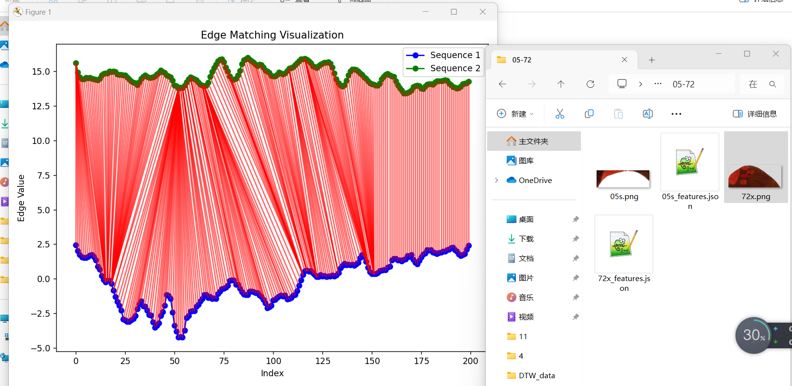
# Plot edge matching visualization with enhanced path
fig, ax = plt.subplots(1, 1, figsize=(8, 6))
# Plot the first sequence (upper edge)
ax.plot(range(len(seq1)), seq1, label="Sequence 1", color="blue", marker='o')
# Plot the second sequence (lower edge) with offset
ax.plot(range(len(seq2)), seq2 + 15, label="Sequence 2", color="green", marker='o') # Offset seq2
# Add alignment path lines with a more precise visualization
for (i, j) in alignment:
ax.plot([i, j], [seq1[i], seq2[j] + 15], color='red', alpha=0.6, lw=1.5) # Offset seq2 and add thickness to lines
# Add legend and title
ax.legend()
ax.set_title("Edge Matching Visualization")
ax.set_xlabel("Index")
ax.set_ylabel("Edge Value")
plt.tight_layout()
plt.show()