


239
社区成员
 发帖
发帖 与我相关
与我相关 我的任务
我的任务
 分享
分享| 这个作业属于哪个课程 | FZU_SE_teacherW_4 |
|---|---|
| 这个作业要求在哪里 | 软件工程实践总结&个人技术博客 |
| 这个作业的目标 | 课程回顾与总结、个人技术总结、软件开发模式 |
| 其他参考文献 | 《构建之法》 |
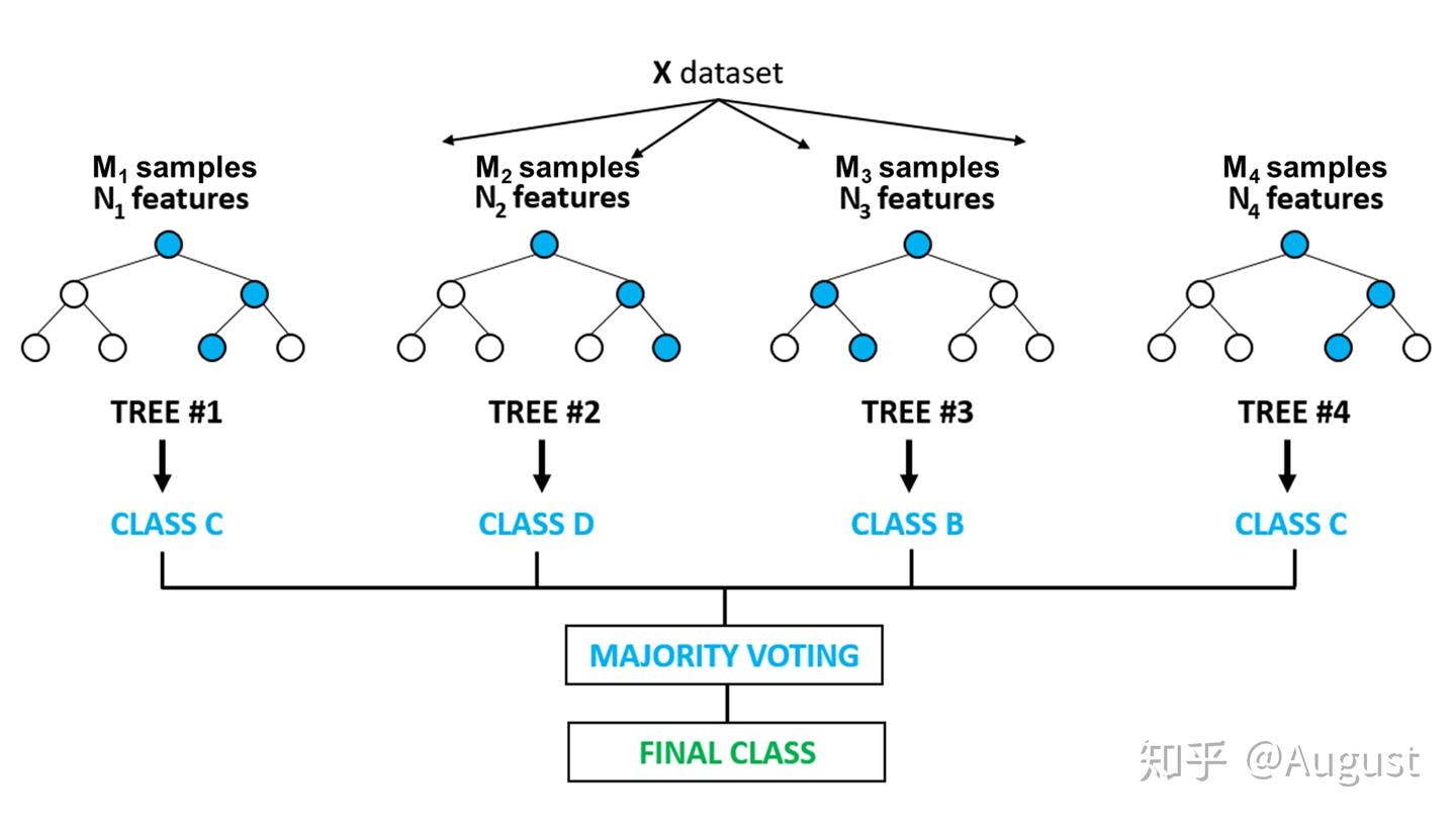
随机森林算法是一种集成学习方法,它通过构建多个决策树并输出平均结果来提高预测准确性和控制过拟合。在分类、回归和特征选择问题中广泛应用,因其出色的性能和易于使用而受到青睐。
学习该技术的原因: 为了实现项目中的赛季选手组别更新算法
难点: 在于调参和理解集成学习背后的原理。
随机森林由多个决策树构成,每棵树在训练时从数据集中随机抽取样本(有放回),以增加模型的多样性。每棵树在构建时,随机选择特征子集进行分裂,最终每棵树独立地给出预测,随机森林通过投票(分类)或平均(回归)来决定最终结果。
对于分类问题,以下是使用sklearn库中的RandomForestClassifier实现随机森林分类器的代码示例:
from sklearn.ensemble import RandomForestClassifier
from sklearn.datasets import load_iris
from sklearn.model_selection import train_test_split

# 加载数据集
iris = load_iris()
X, y = iris.data, iris.target

# 划分训练集和测试集
X_train, X_test, y_train, y_test = train_test_split(X, y, test_size=0.3, random_state=42)

# 创建随机森林分类器实例
rf_clf = RandomForestClassifier(n_estimators=100, random_state=42)

# 训练模型
rf_clf.fit(X_train, y_train)

# 进行预测
y_pred = rf_clf.predict(X_test)
类似地,对于回归问题,可以使用RandomForestRegressor:
from sklearn.ensemble import RandomForestRegressor

# 创建随机森林回归器实例
rf_reg = RandomForestRegressor(n_estimators=100, random_state=42)

# 训练模型
rf_reg.fit(X_train, y_train)

# 进行预测
y_pred_reg = rf_reg.predict(X_test)
随机森林还可以用来评估特征的重要性,这对于特征选择非常有用:
# 获取特征重要性
feature_importances = rf_clf.feature_importances_

# 可视化特征重要性
import matplotlib.pyplot as plt

plt.bar(range(X.shape[1]), feature_importances)
plt.xticks(range(X.shape[1]), iris.feature_names)
plt.show()
以下是sklearn中的随机森林分类器提供的参数
RandomForestClassifier(bootstrap=True, class_weight=None, criterion='gini',
            max_depth=None, max_features='auto', max_leaf_nodes=None,
            min_impurity_decrease=0.0, min_impurity_split=None,
            min_samples_leaf=1, min_samples_split=2,
            min_weight_fraction_leaf=0.0, n_estimators=100, n_jobs=None,
            oob_score=False, random_state=None, verbose=0, warm_start=False)
较多的子树可以让模型有更好的性能,但同时会降低算法的速度。
在保证计算速度的同时,应选择尽可能高的值。
默认决策树在建立子树的时候不会限制子树的深度。
一般数据少或者特征少的时候取默认值。如果样本量多,特征也多的情况下,需要根据数据量和特征量进行设置。常用的取值范围为10-100之间。
这个值限制了子树继续划分的条件,如果某节点的样本数少于min_samples_split,则不会继续再尝试选择最优特征来进行划分。
默认是 2,如果样本量不大,取默认值即可。如果样本量非常大,则增大这个值。
如果某叶子节点数目小于样本数,则会和兄弟节点一起被剪枝。可以输入最少的样本数的整数,或者最少样本数占样本总数的百分比。
默认是1,如果样本量不大,取默认值即可。如果样本量非常大,则增大这个值。
取值为以下几种 (下式中N为样本总特征数) :
auto或sqrt:每颗子树可以利用总特征数的平方根个
。 例如,如果变量(特征)的总数是100,所以每颗子树只能取其中的10个。
“log2”:意味着划分时最多考虑
个特征 。
整数:代表考虑的特征绝对数。 例如 5,就代表选取5个特征。
浮点数 :代表考虑特征总数的百分比。例如0.8表示每个随机森林的子树可以利用特征数为80%*N。
增加max_features一般能提高模型的性能,因为在每个节点上,我们有更多的选择可以考虑。 然而,会降低了单个树的泛化能力,同时降低算法的速度。 因此,你需要适当的平衡和选择最佳max_features。
默认所以的样本权重均为1,当样本类别分布比较均衡时,可以取默认值。当类别非均衡问题比较严重时,需要对该值进行设置,可以设置为"balanced",也可以设置字典{class_label: weight} 来自定义每个类别的样本权重。
这个值限制了叶子节点所有样本权重和的最小值,如果小于这个值,则会和兄弟节点一起被剪枝。
默认不考虑权重。如果我们缺失值较多,或者样本类别非均衡问题比较严重,就需要考虑这个值。
默认不采用袋外数据验证。个人建议设置为True。
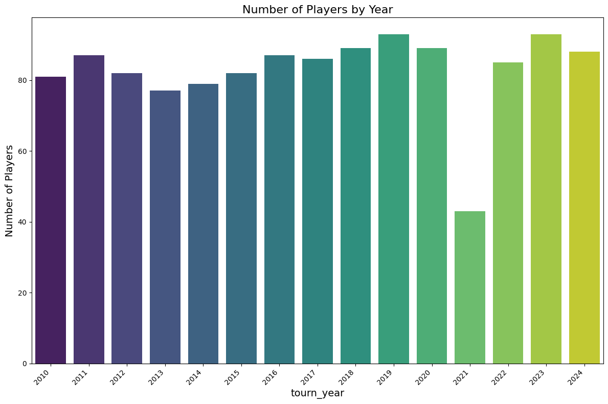
我们训练集数据选取的是男子职业网球选手协会(Association of Tennis Professionals,缩写ATP)的公开网站上2010年到2024年的选手的比赛数据,其中数据字段包括PlayerRank、 PlayerId、PlayerName、PlayerCountryCode、ServeRating、FirstServePct、FirstServePointsWonPct、SecondServePointsWonPct、ServiceGamesWonPct、AvgAcesPerMatch、AvgDblFaultsPerMatch、tourn_year,根据历史经验确定了各组别的人数比例为0.1(大师组), 0.15(钻石组), 0.25(黄金组), 0.5(白银组),按照各组别人数比例为每一年的选手打上标签即当年排名前10%的选手组成大师组,排名前10%-25%的选手组成钻石组,排名前25%-50%的选手为黄金组,25%-75%的选手为白银组,分别对应标签0、1、2、3,基于以上数据,使用随机森林算法可以训练出一个4分类模型,该模型在精确率、召回率、F1-score等指标上都有较高的表现。
具体流程如下:
import pandas as pd

df_atp= pd.read_csv('../data/atp_rankings.csv')
import matplotlib.pyplot as plt
import seaborn as sns

# 统计每个 PlayerCountryCode 的数量
country_counts = df_atp['tourn_year'].value_counts()

# 可视化:条形图
plt.figure(figsize=(12, 8))
sns.barplot(x=country_counts.index, y=country_counts.values, palette='viridis')

# 添加标题和标签
plt.title('Number of Players by Year', fontsize=16)
plt.xlabel('tourn_year', fontsize=14)
plt.ylabel('Number of Players', fontsize=14)

# 旋转x轴标签以防止重叠
plt.xticks(rotation=45, ha='right')

# 显示图形
plt.tight_layout()
plt.show()
df_atp_clean=df_atp.drop(columns=['PlayerRank','PlayerId','PlayerName','PlayerCountryCode'])

import pandas as pd
from sklearn.preprocessing import LabelEncoder
df_atp_clean['FirstServePct'] = df_atp_clean['FirstServePct'].str.replace('%', '').astype(float) / 100
df_atp_clean['FirstServePointsWonPct'] = df_atp_clean['FirstServePointsWonPct'].str.replace('%', '').astype(float) / 100
df_atp_clean['SecondServePointsWonPct'] = df_atp_clean['SecondServePointsWonPct'].str.replace('%', '').astype(float) / 100
df_atp_clean['ServiceGamesWonPct'] = df_atp_clean['ServiceGamesWonPct'].str.replace('%', '').astype(float) / 100


# 计算每一列的均值
mean_values = df_atp_clean.mean()
# 使用均值填充缺失值
df_atp_clean = df_atp_clean.fillna(mean_values)
import pandas as pd
import numpy as np


# 定义比例
proportions = [0.1, 0.15, 0.25, 0.5]

# 为每个 tourn_year 打标签
labeled_data = []

# 遍历每个 tourn_year
for year, year_data in df_atp_clean.groupby('tourn_year'):
    total_rows = len(year_data)  # 当前年份的总行数

    # 计算每个分割的行数
    split_sizes = [int(total_rows * prop) for prop in proportions]
    # 调整最后一个分割的大小,以确保总数加起来等于总行数
    split_sizes[-1] = total_rows - sum(split_sizes[:-1])

    # 为每个分割生成行索引
    indices = np.cumsum(split_sizes).tolist()
    indices = [0] + indices

    # 为每个分割分配标签
    for i in range(len(indices) - 1):
        start, end = indices[i], indices[i + 1]
        split = year_data.iloc[start:end].copy()
        split['Label'] = i  # 标签为0, 1, 2, 3
        labeled_data.append(split)

# 将分割后的DataFrame重新合并为一个
df_atp_labeled = pd.concat(labeled_data).reset_index(drop=True)
from sklearn.linear_model import LassoCV
from sklearn.feature_selection import SelectFromModel
import matplotlib.pyplot as plt
import numpy as np
from sklearn.preprocessing import StandardScaler
import warnings
warnings.filterwarnings('ignore')
# 设置中文字体为黑体,解决中文显示问题(Windows系统下示例,其他系统按需调整)
plt.rcParams['font.sans-serif'] = ['SimHei']
# 解决负号显示问题
plt.rcParams['axes.unicode_minus'] = False
# 特征和标签
X = df_atp_labeled.drop(columns=['Label']) # 特征
y = df_atp_labeled['Label'] # 标签
# 数据标准化
scaler = StandardScaler()
X_scaler = scaler.fit_transform(X)
# 特征名称
feature_names = X.columns
# 初始化 LassoCV,用于自动选择 alpha
lasso = LassoCV(cv=5, random_state=0)
# 拟合 Lasso 模型,找到最佳 alpha 并进行特征选择
lasso.fit(X_scaler, y)
# 使用 SelectFromModel 选择重要特征
model = SelectFromModel(lasso, prefit=True)
X_lasso = model.transform(X_scaler)
# 获取被选中的特征的名称
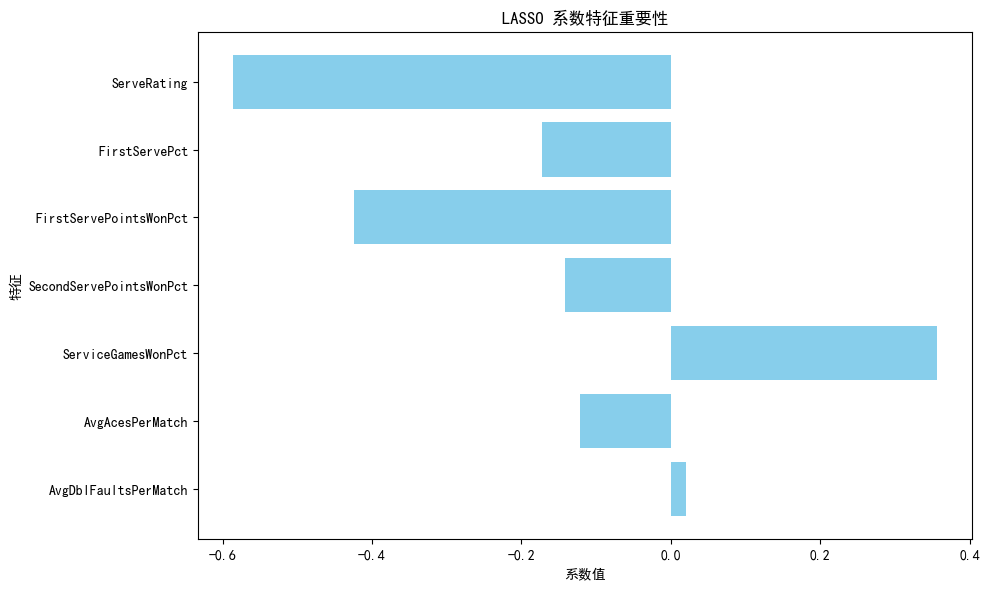
selected_features = [feature for feature, coef in zip(feature_names, lasso.coef_) if abs(coef)>=0.2]
# 输出选择的特征数量
print(f"LASSO 选择了 {len(selected_features)} 个特征,总共 {X.shape[1]} 个特征")
print("LASSO 选择的特征:")
print(selected_features)
# 绘制 LASSO 模型的系数
plt.figure(figsize=(10, 6))
plt.barh(feature_names, lasso.coef_, color='skyblue') # 横向条形图
plt.xlabel('系数值') # x轴标签
plt.ylabel('特征') # y轴标签
plt.title('LASSO 系数特征重要性') # 标题
plt.gca().invert_yaxis() # 将最高系数放在顶部
plt.tight_layout() # 确保布局适应图形区域
plt.show() # 显示图形
from sklearn.model_selection import train_test_split
X_train, X_test, y_train, y_test = train_test_split(X_lasso, y, test_size=0.3, random_state=0)

from sklearn.ensemble import RandomForestClassifier
from sklearn.metrics import accuracy_score, precision_score, recall_score, f1_score
from sklearn.model_selection import GridSearchCV
import numpy as np
import joblib


# 定义要搜索的参数网格,可根据实际情况调整参数及取值范围
param_grid = {
    'n_estimators': [50, 100, 150],
    'max_depth': [None, 5, 10],
    'min_samples_split': [2, 5, 10],
    'min_samples_leaf': [1, 2, 4]
}

# 创建随机森林分类器对象
rf_model = RandomForestClassifier(random_state=0)

# 创建GridSearchCV对象,指定模型、参数网格以及交叉验证的折数(这里设置为5折交叉验证)
grid_search = GridSearchCV(estimator=rf_model, param_grid=param_grid, cv=5,
                           scoring='accuracy', verbose=2, n_jobs=-1)

# 使用训练集数据进行网格搜索
grid_search.fit(X_train, y_train)

# 获取最佳参数组合
best_params = grid_search.best_params_

# 获取最佳模型(在整个训练集上使用最佳参数重新拟合的模型)
best_model = grid_search.best_estimator_

# 在测试集上使用最佳模型进行预测
y_pred = best_model.predict(X_test)

# 计算准确率
accuracy = accuracy_score(y_test, y_pred)

# 计算精确率
precision = precision_score(y_test, y_pred, average='weighted')

# 计算召回率
recall = recall_score(y_test, y_pred, average='weighted')

# 计算F1值
f1 = f1_score(y_test, y_pred, average='weighted')

print("最佳参数组合:", best_params)
print("随机森林模型(最优参数)评估指标:")
print(f"准确率: {accuracy}")
print(f"精确率: {precision}")
print(f"召回率: {recall}")
print(f"F1值: {f1}")
输出结果:
Fitting 5 folds for each of 81 candidates, totalling 405 fits
最佳参数组合: {'max_depth': 5, 'min_samples_leaf': 1, 'min_samples_split': 5, 'n_estimators': 150}
随机森林模型(最优参数)评估指标:
准确率: 0.8900804289544236
精确率: 0.8942139806680881
召回率: 0.8900804289544236
F1值: 0.8894976604433198
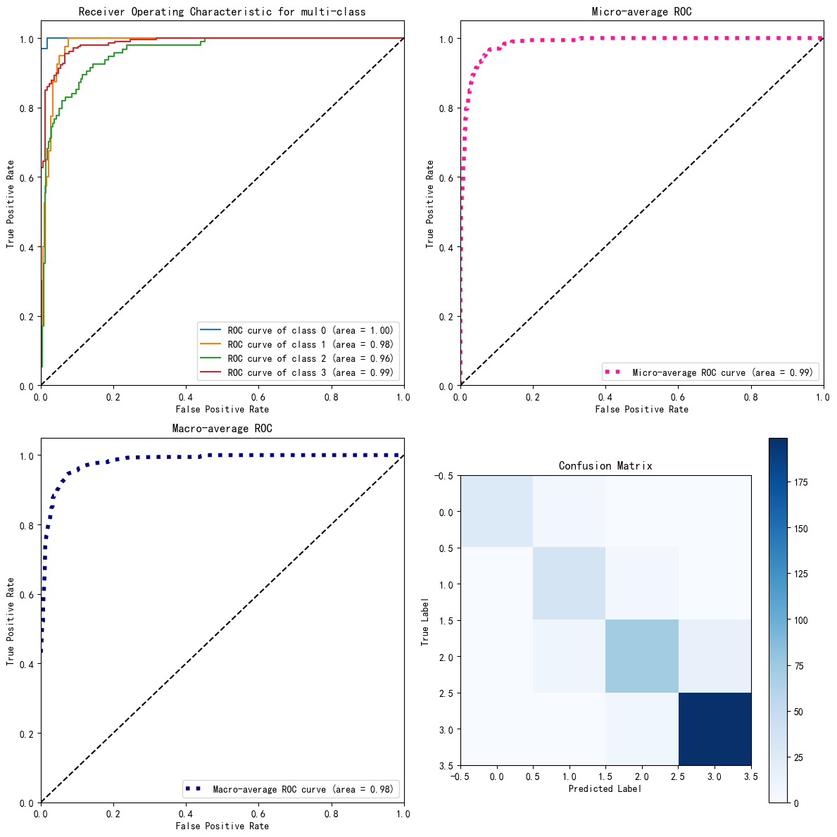
from sklearn.metrics import roc_curve, auc,confusion_matrix
from sklearn.preprocessing import label_binarize
import matplotlib.pyplot as plt
import numpy as np


# Binarize the labels for multi-class classification
y_test_bin = label_binarize(y_test, classes=np.unique(y_test))
n_classes = y_test_bin.shape[1]

# 为每个类别计算预测概率
y_pred_proba_bin = best_model.predict_proba(X_test)

# 计算每个类别的ROC曲线和AUC值
fpr = dict()
tpr = dict()
roc_auc = dict()
for i in range(n_classes):
    fpr[i], tpr[i], _ = roc_curve(y_test_bin[:, i], y_pred_proba_bin[:, i])
    roc_auc[i] = auc(fpr[i], tpr[i])

# 计算微平均和宏平均的ROC曲线和AUC值
fpr["micro"], tpr["micro"], _ = roc_curve(y_test_bin.ravel(), y_pred_proba_bin.ravel())
roc_auc["micro"] = auc(fpr["micro"], tpr["micro"])

all_fpr = np.unique(np.concatenate([fpr[i] for i in range(n_classes)]))
mean_tpr = np.zeros_like(all_fpr)
for i in range(n_classes):
    mean_tpr += np.interp(all_fpr, fpr[i], tpr[i])
mean_tpr /= n_classes
fpr["macro"] = all_fpr
tpr["macro"] = mean_tpr
roc_auc["macro"] = auc(fpr["macro"], tpr["macro"])

# 创建一个2x2的子图布局
fig, axs = plt.subplots(2, 2, figsize=(12, 12))

# 绘制所有类别的ROC曲线
for i in range(n_classes):
    axs[0, 0].plot(fpr[i], tpr[i], label='ROC curve of class {0} (area = {1:0.2f})'.format(i, roc_auc[i]))

axs[0, 0].plot([0, 1], [0, 1], 'k--')
axs[0, 0].set_xlim([0.0, 1.0])
axs[0, 0].set_ylim([0.0, 1.05])
axs[0, 0].set_xlabel('False Positive Rate')
axs[0, 0].set_ylabel('True Positive Rate')
axs[0, 0].set_title('Receiver Operating Characteristic for multi-class')
axs[0, 0].legend(loc="lower right")

# 绘制微平均ROC曲线
axs[0, 1].plot(fpr["micro"], tpr["micro"],
               label='Micro-average ROC curve (area = {0:0.2f})'.format(roc_auc["micro"]),
               color='deeppink', linestyle=':', linewidth=4)

axs[0, 1].plot([0, 1], [0, 1], 'k--')
axs[0, 1].set_xlim([0.0, 1.0])
axs[0, 1].set_ylim([0.0, 1.05])
axs[0, 1].set_xlabel('False Positive Rate')
axs[0, 1].set_ylabel('True Positive Rate')
axs[0, 1].set_title('Micro-average ROC')
axs[0, 1].legend(loc="lower right")

# 绘制宏平均ROC曲线
axs[1, 0].plot(fpr["macro"], tpr["macro"],
               label='Macro-average ROC curve (area = {0:0.2f})'.format(roc_auc["macro"]),
               color='navy', linestyle=':', linewidth=4)

axs[1, 0].plot([0, 1], [0, 1], 'k--')
axs[1, 0].set_xlim([0.0, 1.0])
axs[1, 0].set_ylim([0.0, 1.05])
axs[1, 0].set_xlabel('False Positive Rate')
axs[1, 0].set_ylabel('True Positive Rate')
axs[1, 0].set_title('Macro-average ROC')
axs[1, 0].legend(loc="lower right")

# 绘制混淆矩阵
conf_matrix = confusion_matrix(y_test, y_pred)
cax = axs[1, 1].imshow(conf_matrix, interpolation='nearest', cmap=plt.cm.Blues)
axs[1, 1].set_title('Confusion Matrix')
fig.colorbar(cax, ax=axs[1, 1])
axs[1, 1].set_xlabel('Predicted Label')
axs[1, 1].set_ylabel('True Label')

# 显示图形
plt.tight_layout()
plt.show()
在使用随机森林时,一个常见的问题是模型过拟合。这通常发生在决策树深度过大时。为了解决这个问题,我们可以通过设置max_depth参数来限制树的深度,或者增加min_samples_split和min_samples_leaf参数来提高模型的泛化能力。
随机森林有许多参数需要调整,如n_estimators(树的数量)和max_features(寻找最佳分裂时考虑的特征数量)。我们使用网格搜索(GridSearchCV)来找到最优的参数组合:
from sklearn.model_selection import GridSearchCV

param_grid = {
    'n_estimators': [100, 200, 300],
    'max_features': ['auto', 'sqrt', 'log2']
}

grid_search = GridSearchCV(estimator=rf_clf, param_grid=param_grid, cv=5)
grid_search.fit(X_train, y_train)
随机森林算法因其出色的预测性能和抗过拟合能力而在机器学习领域受到欢迎。通过合理设置参数和理解算法原理,我们可以有效地应用于各种数据集。然而,调参和模型解释仍然是需要关注的问题。通过特征重要性评估,我们可以更好地理解模型的决策过程,并进行特征选择。


