LAB 1-1 individual work

[OuRan偶然]

 

The Link Your Class	https://bbs.csdn.net/forums/MUEE308FZU202201
The Link of Requirement of This Assignment	https://bbs.csdn.net/topics/608734618
The Aim of This Assignment	Self Introduction & Course Planning
MU STU ID and FZU STU ID	MU:20124058    FZU:832001227

 

---

Catalogue

1.self-introduction

2.Skills & evaluating

3.Amount of code

4.Expectations

---

​​​​​​​

1.self-introduction

My name is WENQI PENG, major in Electronic Engineering (EE) in MIEC. What I like is to realize program with my team, it makes me excited and self-confident. In college, I learned a lot of novel knowledge, opened the way to write programs.

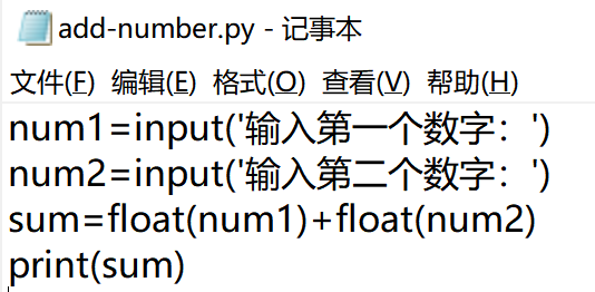
The first language I learned is Python, and of course, the first code is 'print("hello world")'. At that time using codes to solve problems is a really interesting thing for me.

The first program is to add number, which is simple but cool for me at that time.

With the deepening of the course, I learned more knowledge, such as object-oriented, C++, Arduino, and combined software and hardware to make automatic garden irrigation system and intelligent car.

 

2.Skills & evaluating

 1. what professional knowledge I have

• C
• C++
• Python
• Arduino
• Matlab
• Mplab X
• hardware like Single Chip Microcomputer

*The use of SCM knowledge and C++ to do the intelligent freight car

 

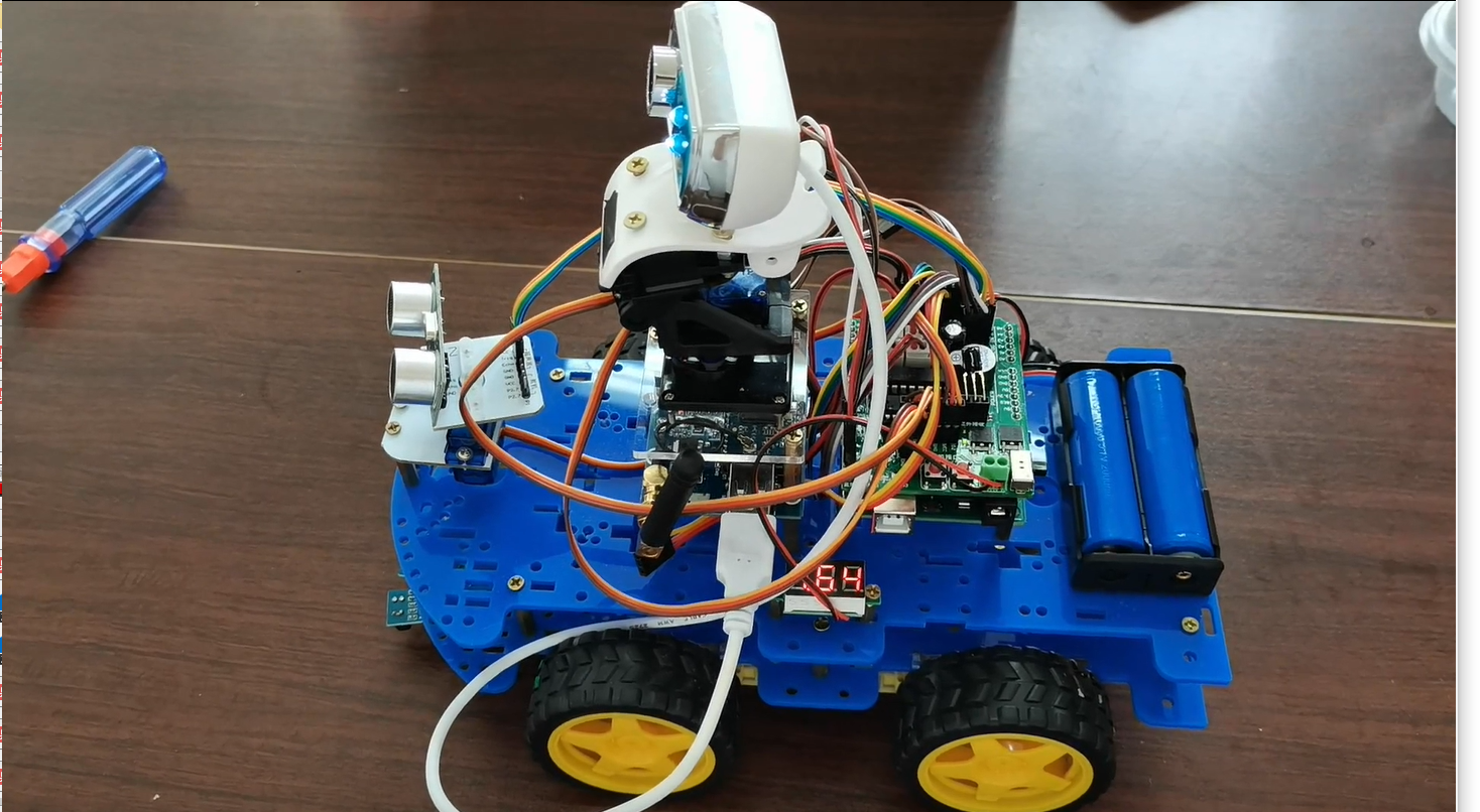
2.what kind of technical direction I am interested in

• web
• mobile terminal

3.which ability I lack of

The ability of knowledge integration is slightly insufficient.

 

3.Amount of code

In fact, as each experiment and study went on, the number of code written could not be calculated clearly.

During the five semesters, the program was written almost every two days, and it was estimated that it had reached 50,000 lines. At the end of this course we hope to add another five thousand lines.

 

4.Expectations

1.What I want to get in this course

In this course, I hope to know the process of software making and have the ability to develop a software together with a team.

 

2.Which role I want to play in this course

In the course of study, I hope to become a serious and hardworking student, a developer with outstanding ability, and a contributor to drive the team forward and guide the direction.

 

---